Introduction Output Screens Input Screens

 Economic Calculations Groundwater Hazard Calculations References

 

 

Pesticide Economic and Environmental Tradeoffs

PEET

by

D.L. Nofziger, A.G. Hornsby, and Dana Hoag

 

 

 

 

Introduction:

 

Controlling pests is an ongoing challenge for farmers.  Farm managers must identify and assess the importance of the pest for their operation.  If they decide some treatment is needed, they often have several treatment options.  This tool is designed to help them evaluate the need for a treatment and select the pesticide treatment. It is an expansion of the work published by Hoag and Hornsby (1992) and Hoag et al., (1994).

 

Farmers have several objectives when managing pests.  One objective is to minimize the economic loss due to the pest.  A second is to protect the environment.  Conflicts sometimes exist between these objectives. Sometimes both can be met without compromise.

 

We developed the Pesticide Economic and Environmental Tradeoffs (PEET) decision-support system to provide information that can help the farmer make these decisions. PEET evaluates the economic benefits of different herbicide treatments for weed control using a weed competition model with user specified weed densities.  A chemical transport model is used to estimate leaching of each active ingredient for the field and management system of interest.  From that, we determine a groundwater hazard index for each treatment.

 

This groundwater hazard index incorporates the amount of pesticide leached and its toxicity.  Results of the economic and groundwater hazard calculations are presented to the user for each potential treatment.  The PEET user can use this information to select the pest management strategy of choice.

 

Economic loss due to weeds for each treatment is determined by estimating the loss in income due to weeds when that treatment is applied plus the cost of the treatment itself.  Losses for each treatment can be compared to losses estimated when no treatment is used.  This shows the user the economic benefits of each treatment. Alternatively the user can view the economic gain associated with a particular weed control practice. (Detailed equations and simplifications used in this calculation are given later in the Calculation of Economic Loss section of this document.)

 

The hazard posed to groundwater by each treatment is defined as the ratio of the concentration of the active ingredient in groundwater to a critical concentration of the active ingredient established for protecting consumers of the groundwater. That is

where GWH is the groundwater hazard, C_{Active Ingredient} is the concentration of the active ingredient in the groundwater, and C_Critical is the concentration of the active ingredient that is considered to have negligible risk of harming human beings when consumed for an entire lifetime. (A description of the model used for this calculation and the simplifications incorporated into it are given later in the Calculation of Groundwater Hazard section of this document.)

 

A groundwater hazard index of 1 (or 100%) means that the calculated concentration of active ingredient in groundwater following a single application of the treatment is equal to the critical concentration for that chemical.  Values less than 1 imply that the concentration of the chemical is less than the critical concentration.  Hazard values greater than 1 correspond to concentrations greater than the critical concentration.  Lower groundwater hazard values imply lower risk of degrading groundwater quality.

 

Sample Output:

Results of the PEET model are available in three forms on the Bar Graphs, Economics/Hazard, and Tables tabs. These are illustrated below for cotton production in Caddo County, Oklahoma.

 

Bar Graphs:

 

 

The figure above presents partial results of a simulation and economic analysis in the form of bar graphs. The list at the center of the figure contains different herbicide treatments and application rates. Additional bars and treatment descriptions for Post-Emergence and Post-Directed treatments can be found by scrolling the actual screen. The bar graph on the left shows the estimated economic gain corresponding to each treatment for the weed species and densities specified by the PEET user assuming a weed-free yield of 800 lb/acre. The length of the bar represents the magnitude of the economic gain for that treatment. The chart on the right shows the groundwater hazard index (on a logarithmic scale) for each treatment. Again the length of the bar represents the groundwater hazard value calculated for this treatment. These values were estimated assuming the field was irrigated at 2 inches per week for the growing season.  The PEET user can use this information to try to select a treatment with a high economic gain and a low hazard.  In some cases this is not possible so tradeoffs must be made.

 

The figure below is an alternative form of the bar graph for the case in which the user has chosen to view the economic loss due to weeds for each treatment instead of the economic gain associated with the treatments. Here bars are also shown for the case in which no treatment is made. The user can observe the impact of different expected weed-free yields by selecting the yield of interest at the top of the screen.

 

 

Economic Gain – Groundwater Hazard Graph: The figure below illustrates another way to view the results. Here the economic gain and groundwater hazard are plotted on the two axes of the graph. The triangles represent different treatments. The treatment associated with each triangle can be viewed by selecting the triangle of interest with the mouse. In this example, the user has selected the triangle in the upper left corner and the system has displayed that treatment in the box under the graph. The preferred treatment option is one that maximizes economic gain and minimizes the hazard. Therefore treatments near the upper left corner of the graph are preferred. This illustration shows results for Pre-Plant Incorporated treatments and an expected yield of 800 lb/acre. Results for other types of application and yields can be shown by selecting other application types and yields on this screen.

 

 

 

Tabular Output: The output of the decision-support system is also available in the tabular form as shown below. Here the treatment type and name are displayed along with the estimated groundwater hazard, economic loss, economic gain, and herbicide cost. This table can be displayed for any of the weed-free yields displayed at the top of the table. The table can also be sorted on any column of the numerical data to view the results in a different sequence. This allows the user to view the treatment options arranged in increasing or decreasing order of economic gain, herbicide cost, or groundwater hazard. Note: Although the gain and loss are displayed to the nearest $0.01 per acre, the model and the  parameters used in estimating these values are not that accurate.

 

 

Some lines in the table shown above include flags. This indicates that special instructions or warnings exist for these treatments. By selecting a particular treatment with the mouse, a screen of the type shown below opens and provides additional information for that treatment. This information can also be obtained for all treatments by selecting the “Details/Warnings” tab on the screen. In addition to warnings about the use of the herbicide and a note that other trade names are available for certain active ingredients, this screen displays the weed densities and competitive load before and after treatment. This information can be used to evaluate the need for subsequent treatments. 

 

 

 

Calculation of Economic Loss:

Calculating the economic loss due to weeds following a specific treatment involves the following steps:

1. Calculate the reduced weed density of each weed in the field following the treatment.
2. Calculate the yield loss due to the reduced weed density
3. Calculate the economic loss due to reduced yield
4. Calculate the cost of the herbicide treatment and its application
5. Find the loss by adding the cost of treatment and the loss due to reduced yield

 

That is

where E_Loss is the economic loss due to weeds after the treatment is applied, Y_Loss is the Yield loss due to weeds, V is the expected market value of the crop, C_Appl is the cost of application of the herbicide, C_Scout is the cost of scouting, m is the number of products included in the treatment, C_Herb and R_Herb are the cost and application rate of each herbicide used in the treatment.

 

The product of the yield loss and the expected market value of the crop represents the loss in income due to reduced crop yield.  The cost of the treatment is the sum of the cost of the herbicides used, the cost of application, and the scouting cost. The total loss is the sum of the loss due to yield and total treatment cost. Since the total loss depends upon the expected yield and that yield is not known in advance, PEET enables the user to enter low, normal and high yields so the economics can be displayed for each of these cases. The user can incorporate results from all of these yields into the treatment decision.

 

The economic gain is defined as the reduction in economic loss resulting from a particular treatment. That is,

 

 

where the economic loss without treatment, E_{Loss without treatment} is simply the product of the yield loss due to weeds for the observed weed density and the expected market value of the crop.

 

The loss in yield due to the weeds must be calculated. Coble and Mortensen (1992) published a model that has been used extensively for this. A basic concept involved is the total competitive load due to weeds. This is a method of calculating the total impact of a mixture of weeds by multiplying the density of each weed species by a weighting factor called the competitive index. The competitive index reflects the relative impact of a single weed of that weed species upon yield loss. The total competitive load D, is given by

 

where c_j represents the competitive index of weed j, d_j represents the density of weed j, and n represents the number of different weed species in the field. The following table illustrates this calculation for weeds.

 

 

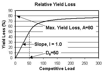
The total competitive load is used to compute the yield loss, Y_Loss, using the equation

 

 

where Y₀ is the expected weed-free yield, D is the total competitive load, I is the slope of the relative yield loss curve for competitive loads less than the threshold value D₀, and A is the maximum relative yield loss at very high values of competitive load. This equation is illustrated below for values of I = 0.01, A = 0.80, and D₀ = 50.

 

 

 

By using the competitive load for no treatment in this equation, we can estimate the yield loss when no treatment is applied.

 

Before the yield loss can be estimated for each possible treatment, we need to estimate the weed density following that treatment. Weed scientists generally evaluate the efficacy of each herbicide on different weeds. The efficacy or fraction of a particular weed controlled by the treatment is used to obtain a reduced weed density for a potential treatment. New values of the competitive load and the corresponding yield loss are then calculated for each treatment. The total competitive load associated with a treatment is given by

where e_j represents the efficacy of the treatment for weed j. Other terms in the equation were defined previously.

 

Data Requirements: Examining the equations above enables us to understand the data required for the economic analysis. Some of those data are provided by the PEET user and some by the weed scientist responsible for implementing PEET for a particular crop and location. The weed scientist will need to provide the name and competitive index of each weed species, a list of potential herbicide treatments, the efficacy of each treatment for each weed, and the parameters used in the yield loss equation. The PEET user must then provide expected low, normal and high yields for the field of interest, names and densities of weeds present in the field, and prices of herbicides, and expected market price of the crop.

 

Data provided by the weed scientist will change frequently as herbicides are introduced or removed and as changes in labels are made. For this reason, PEET is designed to automatically update the software and data each time the scientist changes it on the web server. That means the PEET user will always have access to the latest data. Of course that update feature can only function when the user is connected to the internet. Although PEET can operate without being connected to the internet, we recommend that it be run while connected from time to time so that the data used in the program are kept current.

 

Calculation of Groundwater Hazard:

To determine the groundwater hazard, we must calculate the concentration of each active ingredient in the groundwater.  In general, the amount of chemical leached depends upon soil properties, chemical properties, management practices such as irrigation and tillage, weather, amounts of infiltration, runoff, and uptake of water by plants, the amount of chemical applied, the date of application, and the depth of application.  It is convenient to divide the movement of pesticides to groundwater into three parts. First, the pesticide must be transported from or near the soil surface through the root zone of the soil. Next it must be transported through the underlying vadose zone to the groundwater. Finally it is mixed in the aquifer. The amount of information available for the root zone is greater than for the other two regions so the model used for that component can be more detailed.  Various models exist for estimating the concentration of pesticide in the groundwater. Scientists developing PEET for their location can use the model of their choice.

 

In developing PEET for Oklahoma, we used the CMLS model of Nofziger and Hornsby (1986, 1988) and Nofziger et al (1994) for the root zone and shallow soil. CMLS incorporates biological degradation, sorption on soil solids and the resulting retardation of movement, and mass flow with the soil solution. A simple water balance model is used to estimate water movement. Movement and degradation are calculated daily. We assumed that no degradation of the chemical occurs in the vadose zone. The concentration in the groundwater is estimated by dividing the amount leached beyond the surface soil (usually taken as a depth of 1 meter) by the amount of water present in a saturated soil of specified porosity and specified mixing depth.

 

Since PEET will be used as a decision-aid, we are interested in predicting the future concentration of each active ingredient in the groundwater.  However, leaching losses are highly dependent upon weather (Haan et al., 1994) and we do not know the future weather at a site. Therefore we have uncertainty in the prediction. We believe this uncertainty should be incorporated into the groundwater hazard estimate. To do so, we evaluated the groundwater hazard for many weather sequences each equally likely at each site.  We did this by generating hundreds of weather sequences for each site and simulating movement for each weather pattern.  The collection of results for a particular treatment, soil, and management system were sorted and saved as a probability distribution. Groundwater hazard values displayed by PEET correspond to a probability level chosen by the user.

 

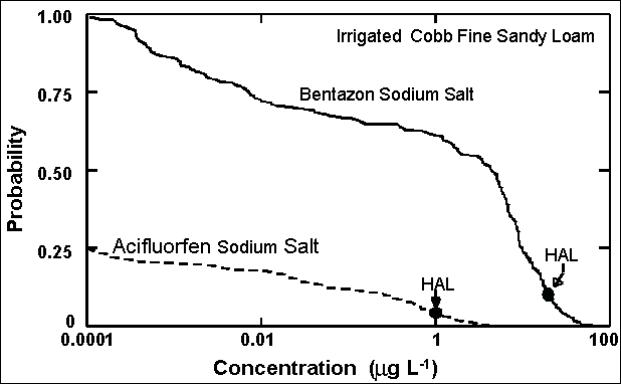
The figure below shows the probability of exceeding different concentrations of bentazon sodium salt and acifluorfen sodium salt in the Cobb fine sandy loam soil.  Note that weather differences produce concentrations ranging from nearly 100 mg L^-1 to less than 0.001 mg L^-1. For the application rates used in this example, bentazon has a much higher probability of exceeding a specific concentration than does acifluorfen. The U. S. EPA lifetime health advisory levels (HAL) for acifluorfen and bentazon are 1 and 20 :g L^-1, respectively, as shown. From the graph we see that the probability of acifluorifen exceeding its HAL is about 0.05 and the probability of bentazon exceeding its HAL is about 0.12.

 

 

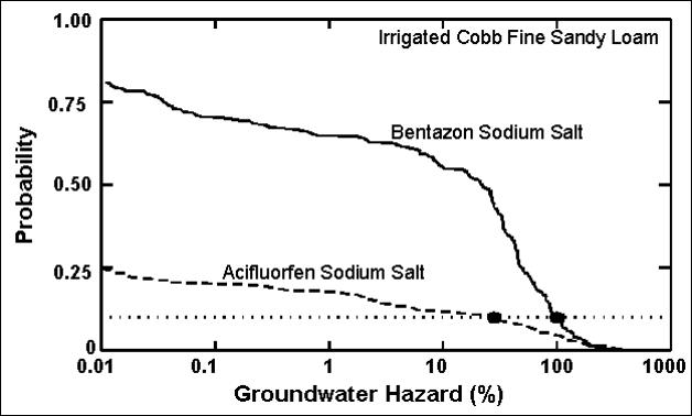
The following figure shows the probability of exceeding different groundwater hazard values for the same two chemicals.  The dotted line represents a probability of 0.10.  The groundwater hazard associated with these two treatments is about 30% for acifluorfen and 100% for bentazon. Acifluorfen appears to pose a lower risk to groundwater quality than bentazon for this soil and these specific conditions.

 

 

Some herbicide treatments involve more than one active ingredient. In those cases, the groundwater hazard is calculated for each active ingredient. The value displayed for those treatments is then the sum of the groundwater hazards for the different active ingredients.

 

Data Requirements: Calculation of the groundwater hazard requires a list of soil names and the soil properties required in the model. For CMLS, these data include the depth, bulk density, organic carbon content, and water content at saturation, field capacity, and permanent wilting points for each soil layer. The calculation also requires the organic carbon partition coefficient, degradation rate, and critical concentration for each active ingredient along with the approximate date at which it will be applied. Hornsby et al. (1996) is a useful source for chemical properties. Daily infiltration and evapotranspiration amounts are also needed. These can be estimated from weather data in CMLS. If irrigation is used, the timing and amount of water applied in this way is also required.

 

Input Screens

 

PEET users specify the needed input parameters in a series of 5 screens labeled with Field/Treatments, Weeds, Economics, Prices, and Options tabs. These are illustrated and discussed below.

 

Field/Treatments: This screen, illustrated below, allows the user to enter a field name and area which are used for identification purposes. Selections of county, soil, irrigation, and tillage are needed for calculating the groundwater hazard. Soil texture and organic carbon content also influences the efficacy of some treatments.  In this example the treatment type chosen was pre-plant incorporated. The results displayed by PEET correspond to the selected type of application and all other types that fall chronologically after the selected type. In this case, the results will be displayed for pre-plant incorporated, pre-emergence, post-emergence, and post-directed spray since the latter 3 are treatment options at the time pre-plant is an option. If post-emergence or post-directed spray are selected, the lower box also requires inputs of the approximate weed size and application date.

 

 

Weeds: This screen is used to enter the density of the weed species present in the field. Since these values are not present for pre-emergence treatments, the user can specify High, Medium, or Low in this column. These values are converted to numeric values using estimates defined in the database by the weed scientist.

 

 

Economics: This screen is used to enter expected yields, expected market price, application costs and scouting costs.

 

 

Prices: This screen is used to enter local prices of different herbicides. Default values are stored in the database, but the user can use this screen to enter actual prices. These values are needed to calculate the treatment cost.

 

 

Options: This screen enables the user to select economic loss or economic gain for the bar graphs and Economics-Hazard graph. In the lower part of the screen, the user can specify the probability level to be used in displaying groundwater hazards, and the mixing depth and porosity of the aquifer underlying the field. In the example below, a probability of 0.05 was selected. This means that if these treatments were applied to this soil under the specified management practices in many different years, the groundwater hazard (estimated using the CMLS simulation model described above) displayed with each treatment would likely to be exceeded only 5 years out of 100. Alternatively, the estimated value of the groundwater hazard is expected to be less than the value presented in 95 years out of 100. The user can also choose to see the groundwater hazard corresponding to the case in which all of the herbicide applied entered the groundwater without degradation. This hazard could be taken as the absolute worst case possible for soils where all of the herbicide moves rapidly to the groundwater through large pores and cracks in the soil. We would not expect this groundwater hazard to be reached as a result of a single application of the herbicide.

 

 

 

 

References

 

Coble, Harold D. and David A. Mortensen.  1992. The threshold concept and its application to weed science.  Weed Technology 6:191-195.

 

Haan, C.T., D.L. Nofziger, and F.K. Ahmed. 1994. Characterizing chemical transport variability due to natural weather sequences. J. Environ. Qual. 23:349-354.

 

Hoag, D.  and A. G. Hornsby. 1992. Coupling groundwater contamination with economic returns when applying farm chemicals.  J. Environ. Qual. 21:579-586.

 

Hoag, D. L., A.G. Hornsby, and D.L. Nofziger. 1994. PEET: Pesticide Economic and Environmental Tradeoffs. Proceedings of the 5^th International Conference on Computers in Agriculture, Orlando FL.

 

Hornsby, A. G., R.D. Wauchope, and A.E. Herner. 1996. Pesticide Properties in the Environment. Springer. New York. 227 p.

 

Nofziger, D.L. and A.G. Hornsby. 1986. A microcomputer-based management tool for chemical movement in soils. Appl. Agr. Res. 1:50-56.

 

Nofziger, D.L. and A.G. Hornsby.  1988.  Chemical movement in layered soils: user's manual. Computer Software Series CSS‑30, Agricultural Experiment Station, Oklahoma State University, Stillwater, OK, and University of Florida.  IFAS. Cir.  780, 44 pp.

 

Nofziger, D.L. J.S. Chen, F. Ma, and A.G. Hornsby. 1994.  CMLS94B Chemical movement in layered soils model for batch processing. Computer Software Series, Oklahoma Agricultural Experiment Station, Oklahoma State University, Stillwater, OK, 76 pp.

 

Developers

D. L. Nofziger, Professor, Department of Plant and Soil Sciences, Oklahoma State University, Stillwater, OK 74078

 

A.G. Hornsby, Professor, Department of Soil and Water Science, University of Florida, Gainesville, FL 93502

 

Dana Hoag, Professor, Department of Agricultural and Resource Economics, Colorado State University, Fort Collins, CO 80523

 

Acknowledgements: The United States Department of Agriculture and the Agricultural Experiment Stations of Oklahoma, Florida, and North Carolina provided funding for this project. The authors want to express appreciation to Dr. Harold Coble, North Carolina State University for assisting with the weed competition component of the program.

 

Contact: D.L. Nofziger at david.nofziger@okstate.edu for more information about this software and its use for other crops and geographic areas.

Last Modified: January 16, 2008.