
CHEMFLO User’s Manual
CHEMFLOTM - 2000
Interactive Software for Simulating
Water and Chemical Movement
in Unsaturated Soils
by
D.L. Nofziger and Jinquan Wu
Department of Plant and Soil Sciences
Oklahoma State University
Stillwater, OK 74078

Table of Contents
Table of Contents..........................................................................iii
Acknowledgements ......................................................................iv
Disclaimer.....................................................................................iv
Purpose of Software......................................................................1
New Features of this Version.........................................................2
Features Retained from Previous Version.......................................2
Limitations of Software..................................................................4
Hardware and Software Requirements...........................................5
Software Installation......................................................................5
Software Use................................................................................8
Graphs..............................................................................9
Reports / Tables..............................................................11
Soil Systems....................................................................12
Initial Conditions..............................................................16
Boundary Conditions.......................................................18
Transport Properties........................................................21
Mesh Size / Convergence................................................22
Examples of Software Use...........................................................24
Water Movement............................................................27
Chemical Transport.........................................................33
Water Movement............................................................36
Chemical Transport.........................................................44
List of Symbols............................................................................50
Numerical Experiments for Water Movement...............................52
Numerical Experiments for Water and Chemical Movement..........63
Related Software.........................................................................68
References..................................................................................69
The authors want to express appreciation to the United States Environmental Protection Agency, the Oklahoma Agricultural Experiment Station, and the Department of Plant and Soil Sciences at Oklahoma State University for funding this work. Joe Williams of the Robert S. Kerr USEPA Laboratory at Ada, Oklahoma, deserves special thanks for his leadership in this project. Thanks are also extended to Mr. Jianbin Yu for his assistance in programming.
Disclaimer
Oklahoma State University, the Oklahoma Agricultural Experiment Station, and the Oklahoma Cooperative Extension Service, hereinafter collectively referred to as "OSU", will not be liable under any circumstances for the direct or indirect damages incurred by any individual or entity due to this software or use thereof, including damages resulting from loss of data, loss of profits, loss of use, interruption of business, indirect, special, incidental or consequential damages, even if advised of the possibility of such damage. This limitation of liability will apply regardless of the form of action, whether in contract or tort, including negligence.
OSU does not provide warranties of any kind, expressed or implied, including but not limited to any warranty or merchantability or fitness for a particular purpose or use, or warranty against copyright or patent infringement.
The entire risk as to the quality and performance of the program is with you. Should the program prove defective, you assume the entire cost of all necessary servicing, repair, or correction.
The mention of a tradename is solely for illustrative purposes. OSU does not hereby endorse any tradename, warrant that a tradename is registered, or approve a tradename to the exclusion of other tradenames. OSU does not give, nor does it imply, permission or license for the use of the tradename.
IF USER DOES NOT AGREE WITH TERMS OF THIS LIMITATION OF LIABILITY, USER SHOULD CEASE USING THIS SOFTWARE IMMEDIATELY AND RETURN IT TO OSU. OTHERWISE, USER AGREES BY THE USE OF THIS SOFTWARE THAT USER IS IN AGREEMENT WITH THE TERMS OF THIS LIMITATION OF LIABILITY.
Purpose of Software:
The movement of water and chemicals into and through soils has a large impact upon our environment and the entire ecosystem. Understanding these processes is of great importance in managing, utilizing, and protecting our natural resources. This software was written to enhance our understanding of the flow and transport processes. It was written primarily as an educational tool. As a result it is highly interactive and graphics oriented. This version of the software expands on that of Nofziger et al (1989) by providing a graphical user interface and other enhancements. The software enables users to define water and chemical movement systems. The software then solves mathematical models of these systems and displays the results graphically.
Water and chemical movement in soils are dynamic processes, changing dramatically over time and space. Soil properties, chemical properties, and water and chemical application rates interact in complex ways within the soil system to determine the direction and rate of movement of these materials. Researchers have worked many years to understand the physical and chemical mechanisms responsible for the movement of these materials. They have developed mathematical models describing these processes and compared the predictions of these models with field and laboratory measurements. The resulting mathematical models form a basis for predicting the behavior of water and chemicals in soils.
This manual presents features of the software, explanations and examples of its use, its limitations, the mathematical equations used to describe the flow and transport systems, and the numerical methods used to solve these equations. The manual also includes a set of numerical experiments that illustrate flow and transport principles and enable users to understand the importance of different soil properties and other physical and chemical factors on water and chemical movement.
The software is intended for use by students, regulators,
consultants, scientists, and persons involved in managing water and
chemicals in soil who are interested in understanding unsaturated flow
and transport processes. We believe this understanding will enhance the
user’s ability to manage our water resources. As is the case with any
model, the user is urged to become familiar with the limitations of the
model and to assess their significance for the situation of interest
before using it for decision-making.
New Features in CHEMFLO – 2000
- Graphical User Interface: This version of CHEMFLO incorporates a new graphical interface. This interface and the tremendous increase in computing power have led to a major change in the software design and operation.
- Enhanced graphics: Graphs have always been an important component of CHEMFLO. This version expands the types of graphs available. Two graphs are displayed at one time to facilitate comparisons. The user selects the parameters of interest from a simple pull-down list. The user also has the ability to show multiple lines on the graphs at one time.
- Capability to perform visual sensitivity analysis: The amount of change in an output parameter resulting from changes in one or more input parameters is important information for judging the quality of data. An analysis of this type is often called a sensitivity analysis. CHEMFLO provides a very convenient method of assessing this sensitivity graphically. The user simply defines and simulates results for one system of interest. The lines representing these results are retained on the screen. The user is then free to change any part of the system to a new value and simulate flow for that system. By comparing the lines on the graphs for the new and old system, the user can observe the impact of the change on the output of interest.
- Improved report generating capability: Report or table formats used in this version are designed to facilitate importing the data into other software for additional analysis or visualization.
- Capability to simulate flow in layered soils: CHEMFLO-2000 supports simulation into layered soils. Although this makes the flow process much more complex, it may be a better representation of real flow systems.
- Support for a new falling head boundary condition representing the infiltration of water into a flooded soil covered with a specified initial depth of water. The water potential at the surface decreases as water enters the soil. Infiltration ends when the water on the surface has entered the soil. Redistribution without evaporation takes place after the surface water has been depleted.
- Improved numerical methods: The numerical methods used for solving the partial differential equations have been improved. The solution to the water flow equation is now carried out to assure that mass balance is maintained. Because of added computer memory, more detailed solutions or solutions for larger systems can be obtained.
Features Retained from Previous Version
- Focus on interactive use as an educational tool: The focus of the software is still interactive use. The user defines a system and views it quickly. He or she then changes the problem of interest and views that result. The graphics screen is now the focus of the entire program.
- Support for non-uniform initial conditions: The software supports flow in soil systems where the initial water content, matric potential, or concentration are not uniform throughout. Convenient tables are used to facilitate defining these non-uniform conditions.
- Support for boundary conditions that change with time: One advantage of solving the flow equations numerically is that boundary conditions can change with time. Support for this is maintained. This permits a user to simulate complex flow systems such as rainfall infiltration followed by evaporation and redistribution.
- Support for a variety of popular models for describing soil properties: Soil properties can be defined using conductivity equations given by Brooks and Corey (1964), Gardner (1958), and van Genuchten (1980). Water characteristic curves can be described using equations of Brooks and Corey (1964), Simmons et al. (1979), or van Genuchten (1980). The editor provided illustrates each equation and common limits for each parameter. It also enables the user to view graphs of these functions.
- Ability to define and store soil properties for future use: Soil properties are stored in an ASCII text table for repeated use. A user can edit these properties for a particular simulation or may save changes permanently as a new soil.
Limitations of Software and Cautions:
1. The models used in this software assume flow and transport in the soil is strictly one-dimensional. Flow in the field will often be multi-dimensional due to layers within the profile, spatial variability of soil properties, and spatially variable application rates (and hence spatially variable boundary conditions).
2. The water flow model does not include any source or sink terms so it cannot simulate plant uptake of water at different depths. Water loss can only occur at the ends of the soil.
3. Inappropriate water flow equation: The Richards equation (Richards, 1931) for water movement is based on the Darcy‑Buckingham equation (Buckingham, 1907) for water movement in unsaturated soils. This equation is usually a good descriptor of water movement in soils, but exceptions exist. No provision is made in the model for swelling soils. No provision is made in this model for preferential flow of water through large pores in contact with free water. Therefore, it will not accurately represent flow in soils with large cracks that are irrigated by flooding. The model assumes that hysteresis in the wetting and drying processes can be ignored. It also assumes that the hydraulic properties of the soil are not changed by the presence of the chemical.
4. Inappropriate chemical transport equation: Limitations in the convection‑dispersion equation have been observed. Clearly, any inadequacy in simulating water movement will impact the simulation of chemicals. In addition, partitioning of the chemical between the solid and liquid phases may not be proportional as assumed here. The model also assumes that this partitioning is instantaneous and reversible. Partitioning and movement of the chemical in the vapor phase is ignored in this model.
5. Inappropriate initial conditions: The simulated results depend upon the initial conditions specified. If the specified initial conditions do not match the real conditions, the calculated values may be incorrect. You may want to analyze the sensitivity of the results of interest to the specified initial conditions.
6. Inappropriate boundary conditions: The predictions of the model can be quite sensitive to the specified boundary conditions. If the specified ones do not match the actual conditions, large errors may be made. In some cases, the errors may be due to a lack of knowledge of the real boundary conditions. In other cases, the software may not be flexible enough to accommodate the real conditions. Hopefully this will not be a major problem since boundary conditions can be changed during a simulation.
7. Inappropriate soil or chemical properties: Many of the soil and chemical parameters are difficult to measure experimentally. Moreover, soil hydraulic properties can vary by large amounts over small areas. This means that the input parameter values involve uncertainty. Repeated simulations with different parameters can be used to assess the influence of this uncertainty upon predictions.
8. Discretization errors: Limitations in the results due to approximating derivatives by finite differences as well as other approximations used in solving the partial differential equations are subtle and are often difficult to detect. Mass balance errors for water and chemicals are calculated to detect net computational error. Small mass balance errors are simply essential conditions for a valid solution, but they do not guarantee accurate solutions. In general, discretization errors tend to decrease as the mesh sizes decrease, so you may want to compare solutions for different mesh sizes.
9. Due to the wide range of flow and transport problems that can be simulated with this software and the highly nonlinear form of the Richards equation, ALWAYS BE ALERT FOR ABNORMALITIES IN THE SOLUTION. If results look suspicious compare the results with those for additional simulations with different mesh sizes. If the solution is important to you, simulate the flow with another model using a different solution method and compare the results.
Hardware and Software Requirements: CHEMFLO-2000 is written in Java[1] 2. Therefore it can be used on any computer system supporting Java 2. This includes Windows 95 / 98 / ME / NT / 2000, Linux, Solaris, and Apple (Mac OS X). Our testing has been primarily on computers running Windows. Differences in fonts across systems result in some problems with the user interface on other platforms.) The software requires at least 64 MB random access memory with 128 MB or more recommended. A fixed disk with 30 MB space is required to install the Java Runtime Environment (which can be used for multiple Java applications). The Java Runtime Environment is available free of charge from Sun Microsystems, Inc. if it is not already built into your operating system. The compiled software and soil data file require less than 1 MB additional disk space. The software is written for a computer with color monitor supporting at least 800x600 pixel resolution.
Software Installation: CHEMFLO-2000 is available in two forms. One is a stand-alone Java application. The second is a Java WebStart1 application. The Java WebStart form is our preferred form since it is easier to install on a computer and can be accessed via a browser when connected to the internet or from an icon on your computer when not connected to the internet. Another advantage of the Java WebStart version is for keeping the software current. Whenever a user starts the program from a computer that is connected to the internet, the system looks at the version of the software on the server from which it was obtained. If the version on the server is newer than the version on the user’s computer, the latest version is downloaded automatically and run. Thus the user can be certain the software being used is the most current version. As is the case with most software, we have plans for adding features to CHEMFLO-2000. Users of the Java WebStart version will automatically obtain these updates while users of the standalone version will need to check the web site and manually download and install any new releases. Another difference in the two forms is that the application has full rights to the user’s computer resources while the Java WebStart form runs in a shell designed to protect your resources. Any requests to use local disk drives or printers must be approved by the user. Another reason for using the Java WebStart form is that we have developed other software utilizing this platform. Once Java WebStart is installed for one application, it can be used by all WebStart applications.
There are three components of the CHEMFLO package. They are the Java software, the CHEMFLO-2000 program, and the user’s manual. These are all available for downloading free of charge. Installation instructions are given below for each component.
- Java Software:
· For the Java WebStart Application: The CHEMFLO software was designed for use with version 1.3.1 (or later) of the Java runtime environment. If the Java WebStart software and 1.3.1 Runtime environment are already installed on your computer you can proceed to step 2. If it is not loaded, you need to download a copy of WebStart and the runtime environment from http://java.sun.com/products/javawebstart/. This is a compressed executable file. After downloading it and saving it in a temporary directory, install it on your computer by running the program. This leads you through the installation process. We suggest that you accept the default values presented by the installation software.
· For the Standalone Application: The CHEMFLO application requires the Java 1.3.1 (or later) runtime environment. If that software is already loaded on the computer to be used, you can skip the remainder of this section and proceed with step 2. If it is not loaded, you need to download a copy of the runtime environment from http://java.sun.com/j2se. This is a compressed executable file. After downloading it and saving it in a temporary directory, install it on your computer by running the program. This leads you through the installation process. We suggest that you accept the default values presented by the installation software.
Note: Versions of Java later than 1.4 include both Runtime and WebStart environments in one package. Installing a late version like this permits the software to be used in both modes.
- CHEMFLO-2000 Software:
-
- The WebStart Application can be downloaded, installed, and run by clicking here.
- The Standalone Application is stored in a zip file about 1.2 MB in size. Press here to download the zip. Save the file in a temporary directory. Extract the files into the Chemflo2000 directory (or another directory of your choice). After unzipping the file, the directory will contain the files listed in Table 1.
Table 1. Contents of chemflo.zip file.
| Name | Contents | |||
|
CHEMFLO.jar |
This file contains the compiled Java program |
|
||
|
Chemflo.bat |
This file is a simple batch file for running CHEMFLO |
|
||
The standalone application program can be executed in several ways.
1. The program can be executed by double clicking on the Chemflo.bat file name from Windows Explorer.
2. The program can be executed by using the Run Chemflo.bat command
3. The program can be executed from an MS DOS command window by changing to the Chemflo2000 directory and issuing the command
java –jar CHEMFLO.jar
4. A shortcut to the Chemflo.bat file can be created and placed on the desktop. The program can then be run by double clicking on this icon.
- Download the CHEMFLO – 2000 User’s Manual in pdf format: This step is needed only if you want to have a local copy of the manual or if you want to print a hard copy of it.
Software Use: The CHEMFLO software is designed for interactive use. When the program comes up a default soil system is already defined and a solution is available. The user can view results for that system or he or she can select an option to define a new system of interest.
The basic steps for simulating water or chemical movement are (1) select or define the soil system; (2) specify the initial conditions for water and chemicals in the soil; (3) define the boundary conditions imposed on the soil system; (4) if chemical movement is being simulated, define the transport properties of the soil – chemical system; and (5) select the graphs option to simulate and view results (or the report option for generating tables).
The opening screen is illustrated below. The upper left corner contains a diagram of the current soil system. In this case it is a vertical soil with a length of 50 cm. Along the left side of the screen are buttons for defining soil systems and viewing results. The panel on the screen changes with each button pressed but the diagram of the soil and the buttons remain in view.
The following pages illustrate and explain the use of each button.
Graphs: This button is likely the
most important one in the program. It produces a panel like the one
below to allow the user to specify the time and position of interest
and to view results in the form of graphs.
Two types of graphs can be drawn. The first type shows the parameter of interest as a function of position along the soil system. This curve is drawn for a specific time. For example, the upper graph in the illustration shows the water content distribution 0.5 hours after flow began for this system. The second type of graph shows the parameter of interest as a function of time for a single position of interest. The lower graph in the figure shows the cumulative flux passing the position x = 0 for all times from 0 to 0.5 hours. Many different graphs are available (see Table 2) and can be selected from the list at the top of each graph. The upper and lower graphs can be used for plotting any combination of graphs of interest.
Data entry cells and scroll bars along the right of the panel are used to specify the time of interest and the position of interest. Press the “Calculate” button after these are entered to simulate movement and draw new graphs. Normally, the current line on the graph will be replaced by a new line for the new time or position of interest. If you want to show more than one line on
the screen at a time, press the “Retain Line” button. The current red line will change colors and the result for the next simulation will be drawn in red. Pressing the “Clear Lines” button removes all lines except the one for the current time and position.
Retaining lines is very useful for making comparisons. For example, I can simulate movement for 1 hour, press the “Retain Line” button, change the time to 2 hours, press the “Calculate” button, change the time to 4 hours and press “Calculate” again. I can then examine distributions of different parameters at these 3 times to gain understanding of how time influences the movement throughout the soil profile. I can also select, calculate, and retain lines for different positions and view graphs of parameter changes with time at these specific positions.
Comparisons of this type are not limited to different times and positions. A user can calculate results for a particular soil and retain that line, change the type of soil and calculate to view the impact of soil type upon movement. In a similar way, a user can compare flow for different initial conditions, different boundary conditions, mesh sizes, chemical properties, etc. This provides us with visual images of the impact of any input parameter upon the output parameter of interest.
Table 2. Graph options available.
Graphs for a Specific Timeand all Positions |
Graphs for a Specific Positionand All Times |
|
· Water Content · Matric Potential · Hydraulic Conductivity (Linear scale) · Hydraulic Conductivity (Semi-log scale) · Driving Force · Flux Density of Water · Total Potential · Water Content vs. Boltzman Variable · Solution Concentration · Total Concentration · Flux Density of Chemical |
· Water Content · Matric Potential · Hydraulic Conductivity (Linear scale) · Hydraulic Conductivity (Semi-log scale) · Driving Force · Flux Density of Water · Total Potential · Cumulative Flux Density · Solution Concentration · Total Concentration · Flux Density of Chemical · Cumulative Flux of Chemical · Mass of Chemical in Soil (per unit area) |
Reports/Tables: The panel illustrated below is used to define tables or reports to be printed, saved as text files, or displayed on the screen. The flow system is defined in the same way as for graphical output. Then the user selects the water and chemical parameters of interest by checking the appropriate boxes. The image shown is for the situation where the user wants to see output for only selected positions and selected times. Those positions and times are entered in the tables at the bottom of the screen. If the user selects output for all positions and selected times, only the left table will be present for entering the desired times. If results are requested for all times and selected positions, the table on the right is used to enter the positions of interest.
When the “Output Table” button is pressed, the user is asked to specify the output device which can be a disk file, the printer, or the screen. Beware: output generated in this option can be very large.
NOTE: Be sure to press the <Enter> key after entering values in the table.
Soil Systems: The
following pages illustrate the screens used to select soils, view and
edit soil properties, view water content and hydraulic conductivity
functions, and define the orientation of the system to be
simulated.
· Select soil: The soil to be used in the simulation is selected by clicking on the soil list and highlighting the soil desired. Properties of the soil are then displayed in the table below. A small list of soils is provided with the software. The user can define and save additional soils.
· Finite or semi-infinite soil: Water and chemical movement can be carried out for soils of finite length made up of 1 to 5 layers. Water movement only can be simulated for homogeneous semi-infinite soils.
· Soil length: If a finite length soil is selected and the soil has only 1 layer, the user can specify the length of the layer here. If the soil has more than one layer, the thickness of each layer is defined as part of the soil definition and can be modified by pressing the “Edit/View Properties button.
· Angle of Inclination: This angle specifies the angle between the increasing x direction and a horizontal line. Zero degrees represents flow in a horizontal system with x increasing to the right; 90 degrees represents a vertical system with x increasing in a downward direction. A diagram of the soil system that is visible from all panels is provided on the main window.
· Delete Soil: Pressing this button brings up a window in which the user can select a soil to be deleted from the file of soils.
· Edit/View Properties: Pressing this button produces a window similar to the one below. Here the properties of the selected soil are displayed and can be edited. In the example shown, the mathematical form of the van Genuchten conductivity function is displayed along with the names and limits for each parameter. This display changes to other conductivity functions and water content functions as the user moves the mouse to different portions of the table below it. Additional layers can be defined by scrolling the properties table, entering the thickness of the next layer (and pressing the Enter key), and then entering the remaining parameters for the layer.
Edit/View Properties Window (Continued):
· OK button: Pressing the OK button saves the current values of soil properties in temporary memory for use in the current simulation. This window is then closed and control returns to the main Soil window.
· Cancel button: Pressing this button cancels the editing just done and returns control to the main Soil window with the original soil properties.
· Store Soil button: Pressing this button brings up a window prompting the user to enter a unique soil name so it can be added to the list of soils saved in a disk file. This enables the user to use the same soil at a later time without entering its properties.
· Draw Graphs button: This opens a new graphics window so the user can view graphs of the water content and conductivity functions as illustrated below. Lower limits for the axis can be modified by clicking the box at the lower left corner of the graph. When a soil contains more than one layer, a line is drawn for each layer.
Initial Conditions: Before making a simulation, the user must define the conditions of water and chemical in the soil before flow begins. These are called initial conditions. The following screens illustrate ways in which these conditions can be defined. The first screen can be used for specifying uniform initial conditions for water flow only. The conditions are specified as uniform matric potential, uniform total potential, or uniform water content. The second screen is used for non-uniform conditions for water flow only. Here the user specifies the initial matric potential or water content for selected positions. The system uses linear interpolation to obtain values for intermediate points.
The following screens can be used when both water and chemical movement are simulated. In the first case, uniform initial matric potential and concentration are specified. In the second case, the initial matric potential is uniform and the concentration is non-uniform. This same format is used when the initial concentration is uniform and matric potential is not uniform or when both are not uniform. Again, linear interpolation is used to obtain values at intermediate positions. The Clear button on the second screen removes all data from the table. The Sort Table button sorts the entries in the table so positions are in increasing order.
Boundary Conditions: Water and chemical movement depends upon the manner in which water and chemical are applied or removed from the soil boundaries. For finite systems, boundary conditions are defined at both ends of the soil. For semi-infinite systems, a boundary condition is needed only at x = 0. The first screen is used to define boundary conditions for a finite soil having a length of 50 cm. The second screen shown below is used for simulating both water and chemical movement in a 50-cm soil.
Time-dependent boundary conditions: CHEMFLO supports flow in systems where boundary conditions change with time. For example, a user may want to simulate water infiltration into a soil for a few hours followed by redistribution and evaporation. This is done in CHEMFLO by defining the first boundary condition and specifying it to begin at t = 0. Flow is then simulated for the number of hours of interest. The user can then return to the Boundary Condition screen and change to a new boundary condition and specify that the simulation should continue with the new boundary condition. This is done by means of the buttons in the upper right corner of each screen. An example of using the software for time-dependent boundary conditions is included in examples of software use.
Boundary conditions at x = 0 supported for water flow include the following:
· Specified matric potential: This boundary condition indicates that the matric potential at x = 0 is maintained at the specified value. For example, a specified value of 2 cm could be used to simulate flow under ponded conditions 2 cm deep.
· Specified total potential: This boundary condition indicates that the total potential at x = 0 is maintained at a specific value. Note: this is actually the same as specifying a matric potential since the reference level in this software always passes through x = 0.
· Specified flux density: This boundary condition identifies the flux density of water at x = 0. The flux is positive in the direction of increasing x. This boundary condition can be used to simulate the flux density of water being pumped into a soil column. It can also be used to simulate water loss from the soil during the constant rate phase of evaporation. One of the most common uses of this is to specify a flux of zero or no water flow at the soil surface.
· Mixed Type: A mixed type boundary condition enables the user to specify a flux density at the soil surface and a critical matric potential. The flux density specified is used at x = 0 until the matric potential reaches the critical matric potential. At that time, the system changes to a constant matric potential boundary condition with a potential equal to the specified critical matric potential. This is useful in simulating both wetting and drying conditions.
· Rainfall rate: This is a mixed type boundary condition with the flux density equal to the specified rainfall rate and the critical matric potential equal to zero.
· Falling head with a specified initial depth of ponding: This boundary condition is a falling head boundary condition where the rate of change in matric potential at the surface is equal to the flux density of water entering the soil. When the matric potential at the surface reaches zero (no more water exists on the soil surface) the boundary condition becomes that of a zero flux density boundary condition.
Boundary conditions at x = 50 cm (or the length of the finite soil system) supported for water flow include the following:
· Specified matric potential: This boundary condition maintains a fixed matric potential at the end of the soil. If the flow is vertically downward, this could be used to simulate flow in a soil with a water table at the bottom of the soil.
· Specified flux density: This maintains a fixed flux density at the end of the soil.
· Free drainage: This boundary condition allows water to flow from a soil column due to a driving force of gravity only. The gradient in matric potential is forced to be zero at this end of the column.
Boundary conditions at x = 0 supported for chemical movement include the following:
· Specified concentration of inflowing solution: By using this boundary condition, a user can specify the concentration of chemical in the solution entering the soil. The flux of solution is the flux of water as determined using the Richards equation. If the flux of water is negative or water is leaving the soil surface, the concentration of chemical in the solution is zero. This boundary condition most realistically represents most flow systems in soils.
· Specified concentration of soil: This boundary condition maintains a specified concentration in the soil solution at x = 0. This is an interesting boundary condition mathematically, but it is difficult to implement experimentally.
Boundary conditions at z = 50 cm (or the length of the finite soil system) supported for chemical movement include the following:
· Convective flow only: This boundary condition specifies that the chemical moves only with the soil solution. Diffusion and dispersion do not contribute to movement at this boundary.
· Specified concentration of soil: This boundary condition maintains the specified soil solution concentration at this boundary.
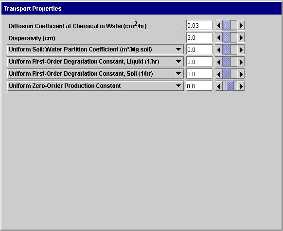
Transport Properties: This screen enables the user to define additional transport properties required for predicting the movement and fate of chemicals in the soil. The example shown below is used when the parameters are uniform across all positions. If one or more parameters vary with position, a table appears and the user enters the position and position-dependent parameters. The uniform values specified are placed in the table automatically.
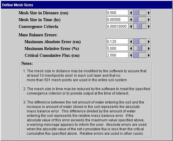
Mesh Size / Convergence: The screen below enables the user to define the preferred mesh sizes, convergence criterion and mass balance parameters. The use and meaning of the terms in it are explained below.
Finite difference techniques are used in this program to solve the partial differential equations for the associated initial and boundary conditions. This method approximates the derivatives in the equations by difference equations in both time and position coordinates. Solutions are then available only at these selected positions and times. The collection of points at which solutions exist are called mesh points. The distance between mesh points is commonly called the mesh size. CHEMFLO uses a uniform mesh size in position within each layer of soil. However, mesh sizes may differ between layers. The solution obtained by this technique depends to some extent upon the mesh sizes used. In general, smaller mesh sizes produce more accurate results.
· Mesh Sizes in Distance: This value determines the distance between points in the x direction. As stated above, it may be modified if needed to accommodate different layer thicknesses or soil lengths. A maximum of 501 mesh points can be used.
· Mesh Size in Time: This value determines the time step used between solutions. It may be reduced by the software to obtain convergence of the Richards equation.
· Convergence Criterion: The Richards equation is highly non-linear. Solving this equation is an iterative process. A criterion must be specified to define convergence of this process. This value determines that criterion. See the section on Computational Methods for Water Movement for a more details on the interpretation of this number.
Mass Balance Errors: Conservation of mass implies that the mass of water accumulating in the soil must be equal to the net amount of water entering the soil system. The difference between these amounts is known as the mass balance error. If the convergence criterion specified above is not sufficiently small, the algorithm can converge but the mass of water is not conserved. The software is designed to warn the user in this case. The final 3 parameters on this screen control when that warning will be displayed.
· Maximum Absolute Error: If the magnitude of absolute mass balance error exceeds this value and the absolute value of the net amount of water entering the soil is less than the Critical Cumulative Flux, the warning will be displayed.
· Maximum Relative Error: If the magnitude of the absolute mass balance error divided by the net amount of water entering the soil exceeds this value and the absolute value of the net amount of water entering the soil is equal to or greater than the Critical Cumulative Flux, the warning will be displayed.
· Critical Cumulative Flux: This value of the net cumulative flux determines whether the absolute or relative mass balance error is used to assess the quality of the numerical solution.
Examples of Program Use:
Scenario #1: Simulate water movement into the default soil when water is applied as rainfall at an intensity of 2.0 cm hr-1 for 8 hours. Consider the soil to be semi-infinite in length, oriented vertically downward, and having an initial matric potential of –500 cm.
The following steps can be used to define the problem and view results:
- Press the “Soil System” button
-
- Select the “Default Soil” from the pull-down list.
- Select a semi-infinite soil
- Set the Maximum Distance to Plot to 80 cm. This sets the upper limit of x on the graphs of different parameters versus distance.
- Set the angle of inclination to be 90 degrees. The diagram of the soil column should be oriented vertically with x = 0 at the top.
- Press the “Initial Conditions” button
-
- Select “Matric Potential” from the pull-down list
- Enter or use the scroll bar to specify a matric potential of –500 cm
- Press the “Boundary Conditions” button
-
- Select “Rainfall Rate” from the pull-down list
- Set the rainfall rate to 2.0 cm hr-1
- In the “Simulations Options” box at the upper right, select “Restart simulation at t = 0.”
- To view results, press the “Graphs” button
-
- Enter the time at which results are desired, for example, 1 hour
- Press “Calculate”
- The current graphs will be updated to reflect the results for this system
- To compare results for several times,
i. Press the “Retain” button (the current line will change colors)
ii. Set the time of interest
iii. Press “Calculate” (a new red line will be drawn for the new time)
- Select different graphs as desired to view different functions of position and time.
Scenario #2: Suppose we want to simulate movement in the default soil after the rainfall stopped in Scenario #1. If no infiltration or evaporation occurs, we can use a boundary condition of zero flux at the soil surface to see how water moves after infiltration stops. The following steps can be used to carry out that simulation.
- Carry out steps 1-3 of Scenario #1
- Press the “Graphs” button
-
- Set the time to 8 hours
- Press “Calculate”
- Press the “Boundary Conditions” button
-
- Select “Flux Density” from the pull-down list
- Set the flux density to zero
- In the “Simulations Options” box at the upper right, select “Continue simulation with new boundary condition”
- Press the “Graphs” button
-
- Set the time of interest to 20 hours (or any other value of interest)
- Press “Calculate”
- View the graphs of interest
Note: The time is not reset to zero when “Continue simulation with new boundary condition” is selected. Thus in this example, the boundary condition imposed from zero to 8 hours is a rainfall boundary condition. The zero flux boundary condition begins at 8 hours and goes to 20 hours (or the value specified in step 4a.)
Scenario#3: Water and chemical movement: Suppose we want to simulate the movement of a non-adsorbed chemical into a soil with irrigation water. Water and chemical were applied at a rate of 1 cm per hour for 2 hours followed by water only for 2 more hours. The chemical has a concentration of 50 g m3 in the irrigation water. It was not present in the soil before irrigation. Where is the chemical after 4 hours of irrigation?
The following steps can be used to carry out that simulation.
- Press the “Soil System” button
-
- Select the “Default Soil” from the pull-down list.
- Select a finite soil
- Specify a length of 100 cm for the soil
- Set the angle of inclination to be 90 degrees. The diagram of the soil column should be oriented vertically with x = 0 at the top and x = 100 at the bottom.
- Press the “Initial Conditions” button
-
- Select uniform matric potential of –500 cm
- Select uniform concentration of 0
- Press the “Boundary Conditions” button
-
- Select “Rainfall” as the water boundary condition at x = 0
- Enter a rainfall rate of 1 cm per hour
- Select “Free Drainage” as the water boundary condition at x = 100
- Select “Specified Concentration of Inflowing Solution” at x = 0
- Enter a solution concentration of 50 g m-3
- Select “Convective Flow” as the chemical boundary condition at x = 100
- Press the “Transport Properties” button
-
- Enter 2 cm for the Dispersivity
- Enter 0 for all other properties
- Press “Graphs”
-
- Select 2 hours as the time of interest
- Select 0 as the position of interest
- Press Calculate
- Observe various graphs of water and chemical. How far did the chemical penetrate into the soil? Where is the leading edge of the chemical?
- Press the “Retain Line” button to save the current lines on the screen
- Press the “Boundary Condition” button
-
- Specify a concentration of 0 for the water entering the soil at x = 0
- In the “Simulations Options” box at the upper right, select “Continue simulation with new boundary condition”
- Press the “Graphs” button
-
- Set the time of interest to 4 hours
- Press “Calculate”
- Observe the water content and chemical distributions
Governing Partial Differential Equation for Water Movement: The partial differential equation used to describe one‑dimensional water movement was published by L. A. Richards (1931) and can be written as
 (1)
(1)
where q =q(h) is the volumetric water content, h = h(x, t) is the matric potential, x is the position coordinate parallel to the direction of flow; t is the time; sin(A) is the sine of the angle A between the direction of flow and the horizontal direction; K(h) is the hydraulic conductivity of the soil at matric potential h; and C(h) is the specific water capacity. That is
![]() (2)
(2)
An angle A of zero degrees corresponds to horizontal flow with x increasing from left to right; an angle of 90 degrees corresponds to vertical flow with x increasing in the downward direction.
Initial Conditions for Water: This software can simulate water movement in soil columns of finite length with uniform or non‑uniform initial conditions. It can simulate water movement in semi‑infinite soils with uniform initial conditions. That is, for a finite soil of length L, the initial condition is
![]() 0 < x <
L
(3a)
0 < x <
L
(3a)
where hinitial(x) is specified by the model user. For the semi-infinite case, the initial condition is
![]() x >
0
(3b)
x >
0
(3b)
where hinitial is a constant specified by the model user.
For convenience, the software allows the user to specify an initial water content or an initial total potential. The software then determines the matric potential for each point for use in equation 3a or 3b.
Boundary Conditions for Water: Three types of boundary conditions can be applied at the soil surfaces. These conditions can be imposed at any time. They may also be changed at any time to simulate complicated flow problems.
At x = 0 the possible boundary conditions are
1. Constant Potential of h0:
![]() (4a)
(4a)
2. Constant flux density of q0:
![]() (4b)
(4b)
3. Mixed Type:
![]() for t £
tc
(4c)
for t £
tc
(4c)
![]() for t > tc
for t > tc
where q0 represents the user-specified flux density at the soil surface (x = 0), h0 represents the user-specified critical matric potential, and tc is the time at which the soil matric potential at x = 0 reaches a value of hc.
4. Falling head:
 (4d)
(4d)
where h0 represents the user-specified ponding depth at the soil surface (x = 0) at time t = 0 and tp represents the duration of ponding.
To facilitate use of the system by inexperienced users, a rainfall boundary condition is included. This is simply a mixed-type boundary condition with q0 equal to the rainfall rate and hc equal to zero.
For a finite soil system, one of the following boundary conditions can be imposed at x = L.
1. Constant matric potential of hL :
![]() (5a)
(5a)
2. Constant flux density of qL:
![]() (5b)
(5b)
3. Free Drainage:
![]() (5c)
(5c)
The Richards equation (Eqn. 1) subject to appropriate initial and boundary conditions defines the water flow problem. The required soil hydraulic properties are defined by specifying the q(h) and K(h) functions. (Forms of equations supported for these functions are shown in Tables 3 and 4.) The solution to equation 1 is h(x, t). From this function and q(h) and K(h) functions, other quantities of interest can be determined. Equations for calculating these quantities are presented on the following pages.
Additional Equations Related to Water Movement:
- Flux density of water: The flux density of water is the volume of water flowing past a certain point in the soil per unit cross‑sectional area (normal to the flow direction) of soil per unit time. It is positive in the direction that x increases and negative in the opposite direction. The flux density of water at the soil surface (x = 0) is positive as water enters this surface and negative as water leaves this soil surface (evaporation). In this model, the flux density of water, q(x, t), is given by the Darcy - Buckingham equation
![]()
or (6)
![]()
where H(x, t) = h(x, t) - x sin(A) is the total potential of the soil water. Sometimes H is called the total hydraulic head.
- Cumulative flux of water: The cumulative flux of water passing position x at time t is the volume of water flowing past position x per unit cross‑sectional area of soil from time t = 0 to the time of interest. This is often used to find the total amount of water flowing past the inlet or outlet of the soil system during the simulation. The cumulative flux, Q(x, t) is given by
![]() (7)
(7)
where q(x, t) is the flux density of water.
- Driving force for water: It is often convenient to view the flux density of water as the product of the hydraulic conductivity and the driving force. Equation 6 implies the driving force, df, is given by
>![]()
 (8)
(8)
- Water content and hydraulic conductivity functions: Mathematical equations for describing soil water content q(h) and hydraulic conductivity K(h) as functions of matric potential are provided in Tables 3 and 4. One function from each table is used to describe the hydraulic properties for each soil layer.
Table 3. Mathematical forms for describing q(h) for soils.
|
||||||||||||||||||
|
|
||||||||||||||||||
|
|
||||||||||||||||||
Table 4. Mathematical forms for describing K(h) for soils.
|
|||||||||||||||
|
|
|||||||||||||||
|
|
|||||||||||||||
Governing Partial Differential Equation for Chemical Movement: Movement and degradation of chemicals in this model is described by the convection‑dispersion equation.
![]() (9)
(9)
where c = c(x, t) is the concentration of chemical in the liquid phase, S = S(x, t) is the concentration of chemical in the solid phase, D=D(x, t) is the dispersion coefficient, q = q(x, t) is the volumetric water content, q = q(x, t) is the flux of water, r = r(x) is the soil bulk density, " a = a(x) is the first-order degradation rate constant in the liquid phase, b = b(x) is the first‑order degradation rate constant in the solid phase, and ( g = g(x) is the zero-order production rate constant in the liquid phase. Here a, b, and g are zero or greater.
If the concentration of the chemical adsorbed on the solid phase is directly proportional to the concentration in the liquid phase, then
![]() (10)
(10)
where k(x) is the partition coefficient. Incorporating equation 10 into equation 9 yields
![]() (11)
(11)
where R is the retardation factor for the chemical in the soil and is given by
![]() (12)
(12)
In this model, the concentration of a chemical in the liquid phase at any location and time is determined by solving equation 11 coupled with equation 1 for water movement. (Values of q(x, t) and q(x, t) from the solution of equation 1 are used in equation 11.) Equation 10 is then used to determine the concentration adsorbed on the solid phase.
Initial Condition for Chemical: This software can be used to simulate chemical movement in soil columns of finite length with uniform or non‑uniform initial conditions. That is, the initial condition is
![]() for 0 < x <
L
(13)
for 0 < x <
L
(13)
where cinitial(x) is specified by the user.
Boundary Conditions for Chemical: Two types of boundary conditions can be imposed at the soil surfaces. These conditions can be imposed at any time. They can also be modified at any time so complex flow problems can be simulated.
The following boundary conditions are supported at x = 0:
- Constant Concentration of Inflowing Solution: This boundary condition is used to simulate movement of chemicals when the solution entering the soil has a known and constant concentration, cs. The amount of chemical entering the soil depends upon the flux of water entering the soil. Moreover, if water is moving out of the soil at x = 0 (as in evaporation), no chemical moves with it. Mathematically, this boundary condition takes the form
![]()
 (14)
(14)
- Constant Concentration in Surface Soil (x = 0): This boundary condition specifies that the concentration c(x, t) at x = 0 is a specified value co. That is
![]() (15)
(15)
Note that equation 15 approximates a system in which the concentration in the soil is abruptly forced to take on a certain value and to remain at that value. This would likely be difficult to carry out experimentally. Equation 14 will likely be a better approximation to real soil systems.
The boundary conditions supported at x = L are described below.
- Convective Flow Only: This boundary condition is used to simulate soil systems in which the chemical moves out of the soil with the moving soil water, but dispersion and diffusion do not contribute to this movement. This condition is equivalent to the requirement that the gradient of the concentration is zero at x = L. That is,
![]() (16)
(16)
- Constant Concentration at Soil Surface (x = L): This boundary condition specifies that the concentration C(x, t) at x = L is a specified value CL. That is
![]() (17)
(17)
Additional Equations Related to Chemical Transport:
- Dispersion coefficient: The dispersion coefficient D at position x and time t is approximated by the equation
![]() (18)
(18)
where l is the dispersivity of the soil-chemical system, D0 is the molecular diffusion coefficient of the chemical in free solution and t is the tortuosity of the soil. The tortuosity is estimated using the equation of Millington and Quirk (1961) where
 (19)
(19)
and qS is the saturated water content of the soil.
- Flux density of chemical: The flux density of chemical at position x is the mass of chemical passing that position in the soil per unit cross‑sectional area per unit time. It is positive in the direction of the x‑axis, as explained for the flux density of water. The flux of chemical, f(x, t), at location x and time t, is given by
![]() (20)
(20)
- The cumulative flux of chemical is the mass of chemical moving past the position of interest per unit cross‑sectional area of soil from time t = 0 to the time of interest. That is, the cumulative flux of chemical, F(x, t) is given by
![]() (21)
(21)
where f(x, t) is the flux density of chemical.
· Total mass of chemical: The total mass of chemical in the soil at time t is the sum of the mass of chemical in the liquid and solid phases. (Partitioning of the chemical to the vapor phase is ignored in this model.) That is,
![]() (22)
(22)
where the mass of chemical in the liquid phase, ml(t), is
![]() (23)
(23)
and the mass of chemical in the solid phase, ms(t), is
![]() (24)
(24)
· Total concentration of chemical: The total concentration, cT(x, t) of chemical in a soil is the sum of the mass of chemical in the soil solution per unit volume of soil plus the mass of chemical adsorbed on the soil solids per unit volume of soil. That is
![]() (25)
(25)
Computational Methods
Flow and transport equations are solved using finite difference methods. That is, difference equations are used to approximate the governing differential equations. To do this, a set of mesh points is defined in the soil. Initial conditions specified by the user determine the values of the matric potential and concentration at these mesh points at time zero. Inserting these values into the difference equations for water movement produces a system of equations (1 equation for each mesh point) that are then solved simultaneously to determine the matric potentials at each point at time t1, a short time later. If chemical movement is being simulated, the initial values and the solution to the water flow equations are used to define a second set of difference equations that are solved for concentration at time t1. These solutions are then used to redefine the water and chemical equations to obtain solutions at a later time, t2. This process is repeated until tj is equal to the time of interest. The following pages contain the details of the equations used.
Water Movement: The computational methods used to solve the Richards equation is based on the work of Celia et al., (1990). This iterative method has the advantage of maintaining mass balance of water.
The backward Euler approximation of equation 1 can be written as
![]() (26)
(26)
where xi, i = 0, 1, 2, …, N represent mesh points in space, and tj, j = 0, 1, 2, … represent mesh points in time. This is a non-linear problem in that the hydraulic conductivity depends upon the matric potential or water content at time tj+1 which is unknown when this equation is applied. Following the work of Celia et al. (1990), we solved this problem using a Picard iteration scheme. In that case, the above equation takes the form
 (27)
(27)
where m represents the iteration number at the current time step. Note that K on the right-hand side is evaluated using iteration m when solving for iteration m+1. The iterations at a single time step are continued until differences between iterations are “sufficiently small”.
Expanding qm+1 with respect to h by Taylor series yields
 (28)
(28)
Inserting equation 28 into 27 and ignoring second order and higher terms yields
 (29)
(29)
where
![]()
 (30)
(30)
The last term in equation 29 was estimated by means of the following difference equation
 (31)
(31)
where xi+1/2 = (xi+1 + xi)/2 and xi-1/2 = (xi + xi-1)/2.
Inserting equation 31 into equation 29 and simplifying yields
 (32)
(32)
for i = 1, 2, 3, …, N-1; j = 0, 1, 2, …; and m = 0, 1, 2, ….
Equation 32, along with 2 additional equations for the two ends of the soil system to be developed later, define the system of N+1 equations to be solved simultaneously. Because this solution is an iterative one, we need to have additional equations to enable us to determine when the difference between solutions for iteration m and m+1 are sufficiently small to allow the process to stop. Celia et al. (1990) derived the needed equations. Equation 29 can be rewritten as
 (33)
(33)
Note that if the right-hand side of this equation is zero, this implies that the solution at iteration m solves equation 27. Therefore these terms can be used to evaluate the residual r and to determine when sufficient iterations have been carried out. Replacing the derivatives on the right-hand side of equation 33 in a manner similar to that in equation 31 and simplifying yields
![]() (34)
(34)
for i = 1, 2, 3, …, N-1. Equation 34 plus 2 additional equations for the ends of the soil column provide equations for determining the residual at each mesh point.
Boundary Conditions at x = 0: Equations for i = 0 must be developed based on the boundary condition imposed. Specified matric potential, flux, and mixed type boundary conditions are supported in this software. Mixed type is simply a combination of the other two so no additional equations are needed for it.
For a specified matric potential of h0 at x = 0 we have
![]() (35)
(35)
for all j and all m. The residual equation in this case becomes
![]() (36)
(36)
To develop the equations for a specified flux q0 at x = 0, equation 1 is written in the form
 (37)
(37)
where q is the flux density of water. The iterative numerical equation for this becomes
 (38)
(38)
where
![]()
 (39)
(39)
Expanding qm+1 in a Taylor series at as done previously and combining with equations 38 and 39 yields
 (40)
(40)
or
 (41)
(41)
The residual equation to be used with equation 41 is obtained by rearranging equation 40. It is
 (42)
(42)
Boundary Conditions at x = L: Equations for i = N must be developed based on the boundary condition imposed. Specified matric potential, flux, and free drainage boundary conditions are supported in this software. The steps involved in deriving these equations are similar to those used at x = 0 so many details will be omitted.
For a specified matric potential of hL at x = L we have
![]() (43)
(43)
for all j and all m. The residual equation in this case becomes
![]() (44)
(44)
For a specified flux qL at x = L we obtain
 (45)
(45)
and
 (46)
(46)
For free drainage at x = L we again begin with equation 37. In this case we have
 (47)
(47)
where
![]() (48)
(48)
and
 (49)
(49)
Inserting the Taylor expansion for qm+1 and simplifying leads to
 (50)
(50)
The residual equation in this case becomes
 (51)
(51)
Calculations and Convergence: Equation 32 and the appropriate equations for the boundary conditions define a set of N+1 linear equations to be solved for each iteration at each time step. The equations can be represented in matrix form where the coefficient matrix is tri-diagonal. As a result, the solution can be obtained quite rapidly and accurately.
The solution process involves the following steps (ignoring logic for cases where convergence fails):
- Utilize the specified initial conditions to initialize h(xi, t0)
- Set time step index j = 1
- Define t1
- While tj is less than or equal to the time of interest
a. Set h0(xi, tj+1) = h(xi, tj)
b. Repeat the following steps until a solution is obtained (Boolean variable called SolutionObtained is true):
i. Set up and solve the system of equations for the current iteration
ii. Set SolutionObtained to true
iii. For each mesh point in the system do the following
1. Calculate the residual using equation 34 (or the alternate equations for nodes 0 and N)
2. If the residual exceeds the critical residual
a. Set SolutionObtained to false
b. Break out of residual calculation loop
c. Save last solution obtained as h(xi, tj)
d. Increment j by 1
e. Define tj
In this program, the solution has converged when
![]() (52)
(52)
for all values of i. Rmax is a number representing the convergence criterion and can be modified by the user (see Mesh Size/Convergence option). Interpreting the physical meaning of Rmax is not straightforward. The default value is 0.0001. It is recommend that users who are concerned about this value examine the sensitivity of the results of interest to different values of this parameter.
In some cases, the system converges slowly or not at all. The
algorithm used reduces the time step if convergence fails after a
predetermined number of iterations. It may later increase it again if
convergence becomes rapid, but it never increases it beyond the value
specified by the user. If reducing the time step several times still
does not result in convergence, the user may be notified and the
calculation stops.
If the value of Rmax is not sufficiently small, the
iterative process may converge based on the criteria above but the
solution may be inaccurate. A mass balance calculation is incorporated
to detect such problems. This mass balance compares the difference
between the quantity of water entering the soil system and that leaving
the soil system with the change in amount stored in the soil.
Conservation of mass implies that these amounts must be equal. If they
are not nearly equal, a warning is issued to the user who can then
choose to use a smaller value of Rmax and / or smaller mesh
sizes.
Chemical Transport : The preceding section presents the equations and logic for solving the water flow equation. If chemical transport is being simulated, the system sets up and solves the transport equations at each time step (before incrementing j and defining a new tj in the previous outline of calculations.) The flux density and water content at each point are used in the solution to equation 9 for that time step. This alternating solution process continues until the time of interest has been reached.
The numerical solution to equation 9 is based on that of van Genuchten (1978). In that work, he derived a correction for numerical dispersion. The equations used in that work are outlined below. An equation is derived for each mesh point in position. Values of concentration for time t0 are determined from the initial conditions. This system of equations is solved simultaneously to obtain the concentration at all points for time t1. Since no more than 3 mesh points are involved in any single equation, the coefficients of the unknown concentrations form another tri-diagonal matrix that can be readily solved. The equations are linear in this case so no iteration is required.
The following equations define the system of equations that are solved for each time step. Equations 53-59 define the equations for the interior mesh points or for xi for i = 1, 2, 3, …, N-1.
 (53)
(53)
where
![]() (54)
(54)
 (55)
(55)
 (56)
(56)
 (57)
(57)
 (58)
(58)
![]() (59)
(59)
and xi for i =0, 1, 2, …, N are mesh points in position and tj for j = 0, 1, 2, … are mesh points in time. Equation 53 can be applied to mesh points xi for i = 1, 2, 3, …, N-1 and all values of j. Additional equations needed at the boundaries of the soil system (x0=0 and xN=L) are given below.
Boundary condition #1 at x = 0 - Specified concentration of inflowing solution: Equation 53 can be written as
 (60)
(60)
where
![]() (61)
(61)
 (62)
(62)
 (63)
(63)
 (64)
(64)
![]()
![]() (65)
(65)
Equation 60 in combination with equations 61-65 provides the equation for the first mesh point with this boundary condition.
Boundary condition #2 at x = 0 – Specified concentration of soil solution: This condition given in equation 15 implies
![]() (66)
(66)
where x0 = 0, j = 0, 1, 2, …, and t0 = 0. This provides the relationship for the first equation with this boundary condition.
Boundary Condition #1 at x = L – Convective Flow Only: Again we can write equation 53 as
 (67)
(67)
![]() (68)
(68)
 (69)
(69)
![]() (70)
(70)
 (71)
(71)
![]() (72)
(72)
Equation 67 in combination with equations 68-72 provide the equation for the first mesh point with this boundary condition.
Boundary Condition #2 as x = L – Specified concentration of soil solution: This condition given in equation 17 implies
![]() (73)
(73)
The equations above form a system of N+1 simultaneous equations that are solved for the solution concentration at the mesh points, xi and time tj+1 . The equations take to form
 (74)
(74)
for i = 1,2,3, …, N-1 where
 (75)
(75)
 (76)
(76)
 (77)
(77)
and
 (78)
(78)
For i = 0 and a specified concentration of the inflowing solution, the equation is
 (79)
(79)
where
 (80)
(80)
 (81)
(81)
and
 (82)
(82)
Note: If q(x0,t) is zero or less than zero, the last term in equation 79 drops out.
For i = 0 and the specified concentration at x = 0, the equation is
![]() (83)
(83)
For the convective flow boundary condition at x = L we obtain the following equation for i = N.
 (84)
(84)
where
(85)
(86)
and
 (87)
(87)
For a specified soil solution concentration at x = L the equation is
![]() (88)
(88)
Table 5. List of symbols,
descriptions and units used in text.
Symbol |
Description |
Units |
|
A |
- angle between the direction of flow and the horizontal direction |
degrees |
|
C(h) |
- specific water capacity, dq/dh |
cm-1 |
|
c(x,t) |
- concentration of chemical in the soil solution at position x and time t |
g m-3(water) |
|
cT(x,t) |
- total concentration of chemical in the soil at position x and time t |
g m-3(soil) |
|
cinitial(x) |
- initial concentration of chemical in solution at t = 0 |
g m-3(water) |
|
cs |
- concentration of inflowing solution at x = 0 for constant concentration of inflowing solution boundary condition |
g m-3(water) |
|
c0 |
- concentration of soil solution at x = 0 for constant concentration boundary condition |
g m-3(water) |
|
cL |
- concentration of soil solution at x = L for constant concentration boundary condition |
g m-3(water) |
|
D(x,t) |
- dispersion coefficient of chemical in soil at position x and time t |
cm2 hr-1 |
|
D-, D+ |
- dispersion coefficients corrected for numeric dispersion |
cm2 hr-1 |
|
D0 |
- molecular diffusion coefficient of chemical in free solution |
cm2 hr-1 |
|
df |
- driving force for water, -¶H/¶x |
- |
|
F(x,t) |
- cumulative flux of chemical passing position x at time t |
g m-2 |
|
f(x,t) |
- flux density of chemical at position x and time t |
g m-2 hr-1 |
|
H(x,t) |
- total soilwater potential (or total hydraulic head) at position x and time t |
cm |
|
h(x,t) |
- matric potential at position x and time t |
cm |
|
hinitial(x) |
- initial matric potential function at t = 0 for finite length soils |
cm |
|
hinitial |
- initial matric potential at t = 0 for semi-infinite soil |
cm |
|
h0 |
- matric potential at x = 0 for constant potential or mixed type boundary condition |
cm |
|
hL |
- matric potential at x = L for constant potential boundary condition |
cm |
|
i |
- index of mesh points in position |
- |
|
j |
- index of mesh points in time |
- |
|
K(h) |
- soil hydraulic conductivity at matric potential h |
cm hr-1 |
|
KS |
- saturated hydraulic conductivity |
cm hr-1 |
|
k(x) |
- partition coefficient of chemical in soil at position x |
m3 Mg-1 |
|
L |
- length of soil column |
cm |
|
m |
- index of iteration number in solving flow equation |
- |
|
ml(t) |
- mass of chemical in soil solution per unit cross-sectional area |
g m-2 |
|
mS(t) |
- mass of chemical adsorbed on soil solids per unit cross-sectional area |
g m-2 |
|
mT(t) |
- total mass of chemical in soil system per unit cross-sectional area |
g m-2 |
|
Q(x,t) |
- cumulative flux of water passing position x at time t |
cm |
|
q(x,t) |
- flux density of water at position x and time t |
cm hr-1 |
|
q0 |
- constant flux density at x = 0 for constant flux or mixed type boundary condition |
cm hr-1 |
|
qL |
- constant flux density at x = L for constant flux boundary condition |
cm hr-1 |
|
R |
- retardation factor for chemical in soil |
- |
Table 5. (Continued)
Symbol |
Description |
Units |
|
Rmax |
- convergence criterion used in solving flow equation |
- |
|
ri |
- residual at mesh point i in solution to flow equation |
hr-1 |
|
S(x,t) |
- concentration of chemical adsorbed on the solid phase at position x and time t |
g Mg-1 |
|
t |
- time |
hr |
|
tc |
- time at which mixed type boundary condition changes from flux type to potential type boundary condition |
hr |
|
x |
- position coordinate in the direction of flow |
cm |
|
a(x) |
- first-order degradation rate constant in liquid phase at position x |
hr-1 |
|
b(x) |
- first-order degradation rate constant in solid phase at position x |
hr-1 |
|
g(x) |
- zero-order production rate constant in liquid phase at position x |
g m-3 hr-1 |
|
q(h) |
- volumetric water content of soil at matric potential h |
m3 m-3 |
|
q(x,t) |
- volumetric water content at position x and time t |
m3 m-3 |
|
qs |
- saturated volumetric water content |
m3 m-3 |
|
r(x) |
- soil bulk density at position x |
Mg m-3 |
|
t |
- soil tortuosity |
- |
|
l |
- dispersivity |
cm |
Numerical Experiments For Water Movement
ADVANCE \u 7
1. Infiltration of Water Ponded on the Soil Surface
|
Objective: |
1. To determine the nature of the dynamic infiltration process for water ponded on the soil surface. 2. To compare the infiltration rate at different times with the saturated hydraulic conductivity of the soil.
|
|
Situation: |
Water is applied to a loam soil by flooding the soil to a depth of 2 cm. Water is continually applied to the soil surface to maintain this height of water. The soil was somewhat dry throughout before the water was applied. We want to observe the rate at which water enters the soil and the total amount entering the soil.
|
|
Simulation: |
Simulate water movement into a vertical semi‑infinite loam with an initial matric potential of ‑2000 cm. Apply water to the soil at a constant potential of 2 cm. Simulate movement for 12 hours. Display the flux of water at the soil surface and the cumulative infiltration of water as functions of time.
|
|
Additional Work: |
Repeat the above exercises for different soils. Compare the infiltration rates and the saturated hydraulic conductivities. Are the results consistent with those above? |
Numerical Experiments For Water Movement
2. Infiltration of Water From Rainfall or Sprinkler Irrigation
|
Objective: |
1. To determine the nature of the dynamic infiltration process for rainfall or sprinkler irrigation. 2. To compare the infiltration rate at different times with the saturated hydraulic conductivity of the soil. 3. To determine the total amount of infiltration, the total amount of runoff, and the time at which runoff occurs
|
|
Situation: |
A farmer recently irrigated his field so that the soil was relatively wet. Unexpectedly, a rainstorm occurred. The storm lasted for 6 hours. The rainfall rate was 0.75 cm/hr. The field was a silt loam soil. How much of the rain water entered the soil? Did any runoff occur? If so, how much? When did runoff begin?
|
|
Simulation: |
Simulate water movement into a vertical semi‑infinite silt loam soil with an initial matric potential of ‑100 cm. Apply water to the soil at a rainfall rate of 0.75 cm/hr. Simulate movement for 6 hours. Display the flux of water at the soil surface and the cumulative infiltration of water as functions of time.
|
|
Additional Work: |
Retain the lines for the graphs used above. Then decrease the saturated conductivity of the soil by 0.1 cm/hr and repeat the simulation. Compare the sets of curves. Did the reduction of saturated conductivity have much impact upon the time at which runoff began or on the total amount entering the soil?
Repeat the exercise with different rainfall rates. How does rainfall rate influence the time at which runoff begins and the total amount entering the soil in the 6 hour period? |
.
Numerical Experiments For Water Movement
ADVANCE \u 7
- Water Content and Matric Potential Distributions During Infiltration
|
Objective: |
1. To observe water content and matric potential distributions during infiltration at selected times
2. To observe changes in water content and matric potential with time at selected distances from the inlet.
3. To compare the distributions for infiltration due to ponding with those due to infiltration of rainfall
|
|
Situation: |
The settings are similar to those described in the preceding exercises. However, in this case there is an interest in the behavior of the water within the soil profile, not just the rate at which it enters the soil.
|
|
Simulation: |
Simulate water movement into a vertical, semi‑infinite silt loam soil with an initial matric potential of ‑2000 cm.
Distributions at selected times: 1. Apply water to the soil at a constant potential of 2 cm as done in exercise 1.
A. Set the time of interest to 0 and press the calculate button. Display graphs of water content versus distance and matric potential versus distance. These graphs represent the water content and matric potential at time zero or before flow begins.
B. Increase the time of interest by 1 hour, retain the line, and calculate again. Observe the change in water content and matric potential graphs. Note that the soil water content and matric potential change only to a certain depth. Below that depth, the parameters retain their initial value. This indicates that water movement has penetrated through only part of the soil. Record the depth of wetting for each hour for 12 hours. Does the wetting depth increase uniformly with time or does it appear to slow down? Why?
C. Observe the water content at the soil surface (distance = 0). What is its value? Does the value change with time when the water is applied by ponding?
D. Compare the shape of the water content profiles with those of the matric potential profiles. Remember that these curves are related to each other by means of the water release or water characteristic curve.
2. Repeat the simulation for the same soil with the same initial condition but with water applied as rainfall at an intensity of 0.5 cm/hr. Compare these results with those found in part 1. Take special note of changes in water content near the soil surface.
|
3. Water Content and Matric Potential Distributions During Infiltration (Continued)
|
Simulation Continued: |
Distributions at specific locations: 1. Using the same initial conditions as earlier in this experiment, simulate movement for 12 hours with position of interest set to zero. Select graphs of water content vs. time and matric potential vs. time. Press the button to retain these lines. Then repeat the simulation for a position of interest equal to 5 cm. Retain these lines as well. Finally simulate a third time for a position of interest equal to 10 cm. These sets of curves illustrate the way the water content and matric potential change with time at each location.
A. Observe the curves for the three depths. What similarities and differences do you find?
B. In general, the water content at a specific location remains at its initial value until water reaches that depth. It then increases. At what time does the water content begin to increase at 0, 5, and 10 cm? Does it take longer for the water to move from 5 cm to 10 cm than it took for water to move from 0 to 5 cm?
C. Compare the slope of the water content vs. time graphs for the three depths. Which depth shows the most rapid change? Which changes least rapidly?
2. Repeat the simulation for the same soil with the same initial condition but with water applied as rainfall at an intensity of 0.5 cm/hr. Compare the times at which water content changes occur and the slopes of the curves for water applied by ponding with those values for water applied as rainfall. What differences do you observe? Why?
|
|
Additional Work: |
Determine the time at which runoff began for the simulation with water applied as rainfall. What was the value of the water content at a depth of zero at that time? What was the value of the matric potential at that time? Formulate an hypothesis about the relationship between these parameters and test that hypothesis |
.
.
Numerical Experiments For Water Movement
ADVANCE \u 7
4. Comparison of Horizontal and Vertical Water Movement in Unsaturated Soils
|
Objective: |
1. To compare the water movement in horizontal and vertical soil systems.
2. To assess the significance of the force of gravity in unsaturated water movement.
|
|
Situation: |
Water is applied to a silt loam soil by means of furrow irrigation. The field was irrigated for 10 hours. The farmer noticed that the soil surface between the furrows became wet rather quickly. The farmer wanted to compare the distance the water moved horizontally with the distance it moved vertically downward. |
|
Simulation: |
Simulate water movement for 1 hour into a vertical semi‑infinite soil with an initial matric potential of ‑2000 cm. Apply water to the soil at a constant potential of 1 cm. Observe the water content as a function of distance from the inlet and the cumulative flux of water passing the inlet. Retain these lines. Change the orientation of the column so the soil is oriented horizontally. Calculate the flow for this system.
1. How far did the water move in each direction? (Choose a water content in the middle of the range and determine the depth to which that water content penetrated.)
2. Compare the flux of water at the soil surface (the infiltration rate) for the two cases.
3. Compare the cumulative infiltration in both cases.
4. Compare the driving forces for the two systems.
5. Repeat the simulation for 2, 4, 6, 8, and 10 hours and make the observations suggested above. What trends do you observe as time increases?
6. Why does water move horizontally nearly as fast as vertically?
|
|
Additional Work: |
Repeat the above exercises for a sandy clay loam and a sandy loam soil. What similarities and differences do you observe?
Repeat the experiments for soils that are initially wetter. For example, choose an initial matric potential of ‑200 cm and repeat the experiments. Are the results consistent with those above?
These simulations compare vertically downward and horizontal water movement. You might want to compare vertically downward, horizontal, and vertically upward flow. What do you expect to see? Do the simulations support your expectations? |
Numerical Experiments For Water Movement
ADVANCE \u 7
5. Redistribution of Soil Water following Infiltration
|
Objective: |
To observe movement of water within a soil profile after infiltration has taken place but in the absence of evaporation. |
|
Situation: |
A scientist flooded a plot of loam soil by maintaining 5 cm of water on the surface for 6 hours. At that time, borders were opened and the water quickly flowed off the soil surface. Then the surface was covered with plastic and insulated to prevent evaporation. If the soil had an initial matric potential of ‑1000 cm at all depths, what will be the distribution of water at the time infiltration stopped? How will this distribution of water change during the next 5 days while the plot is covered? |
|
Simulation: |
Simulate water infiltration into a vertical semi‑infinite loam soil with an initial matric potential of ‑1000 cm. Water was applied by flooding the soil surface to a depth of 5 cm for 6 hours. At that time, the surface was covered so no infiltration or evaporation took place. This is simulated by specifying a constant flux boundary condition of zero at the soil surface beginning at 6 hours. This zero flux boundary condition should continue until the simulated time reaches 120 hours. Answer the following questions using graphs of water content profiles, matric potential profiles, and water content vs. time.
1. Describe the water content profiles during the redistribution process. In what ways do they differ from profiles observed during infiltration?
2. What was the depth of wetting when infiltration stopped? What was the depth of wetting at 12, 24, 48, 72, 96, and 120 hours?
3. What changes in water content and matric potential occurred in the soil near the surface?
4. Does movement continue beyond 2 days? When will movement stop?
5. Why does the rate of water movement decrease as redistribution time increases?
|
|
Additional Work: |
Conduct additional experiments to determine if the observations made above can be generalized for other soils, wetting times, and initial conditions.
|
Numerical Experiments For Water Movement
ADVANCE \u 7
6. Redistribution and Evaporation of Soil Water following Infiltration
|
Objective: |
To observe the simultaneous downward redistribution and upward evaporation of water within a soil profile after infiltration.
|
|
Situation: |
A field of a loam soil was flooded by maintaining 5 cm of water on the surface for 6 hours. At that time, the water was removed from the soil surface. If the soil had an initial matric potential of ‑1000 cm at all depths, what was the distribution of water at the time infiltration stopped? How will this distribution of water change during the next 5 days.
|
|
Simulation: |
Simulate water infiltration into a vertical semi‑infinite loam soil with an initial matric potential of ‑1000 cm. Water is applied by flooding the soil surface to a depth of 5 cm for 6 hours. At that time, evaporation and redistribution will take place. Suppose the atmospheric conditions are capable of evaporating 0.05 cm of water per hour as long as water is available at the surface for evaporation. After that time, the soil limits the evaporation rate. This scenario is simulated by specifying a mixed type boundary condition at the surface beginning 6 hours after flooding. Set the flux to ‑0.05 cm/hr and the critical matric potential at the soil surface to ‑5000 cm. This mixed type boundary condition should continue until 120 hrs have been simulated. Answer the following questions using graphs of water content profiles, matric potential profiles, and water content vs. time.
1. Describe the water content profiles during the evaporation and redistribution process. In what ways do they differ from profiles observed during infiltration? How does the evaporation process change the curves?
2. What was the depth of wetting when infiltration stopped? What was the depth of wetting at 12, 24, 48, 72, 96, and 120 hours?
3. What changes in water content and matric potential occurred in the soil near the surface?
4. What is the evaporation rate from the soil surface? Does it change with time? Explain. (The evaporation rate is the flux of water at a depth of zero. This number will be negative since it is upward.)
5. What is the total amount of water lost to evaporation during the 120 hours?
6. Why does the rate of water movement decrease as time increases?
|
|
Additional Work: |
Design and carry out additional experiments to determine the influence of the initial evaporation rate upon the duration of the "constant rate" phase of the evaporation process and upon the total amount of water lost to evaporation during the 120-hour period.
Conduct additional experiments to determine if the observations made above can be generalized for other soils, wetting times, and initial conditions. |
Numerical Experiments For Water Movement
ADVANCE \u 7
7. Influence of Rainfall Rate upon Infiltration and Depth Wetting
|
Objective: |
To determine the influence of rainfall rate upon the infiltration rate, time to runoff, and depth of wetting |
|
Situation: |
A farmer has the option of applying water by sprinkler irrigation at different rates. He would like to know if the rate of application affects the way the soil wets and the amount of water entering the soil. He wants to try irrigating the sandy loam soil at 0.25, 0.5, 1.0, and 2.0 cm/hr. In each case he will apply 4 cm of water. The soil before irrigation has a matric potential of ‑1000 cm. |
|
Simulation: |
Simulate water infiltration into the vertical sandy loam soil for a rainfall rate of 0.25 cm/hr for 16 hr. Observe the infiltration rate, depth of wetting, and total infiltration. Calculate the amount of runoff, if any. Repeat the simulation for a rainfall rate of 0.5 cm/hr applied for 8 hr, 1.0 cm/hr applied for 4 hr, and 2 cm/hr applied for 2 hr. Answer the following questions:
1. What was the total amount of water entering the soil at each rate?
2. What was the amount of runoff?
3. Did the application rate affect the form of the wetting process and the depth of wetting in the soil? If so, how?
4. Should the farmer be concerned about the rate of irrigation? Explain your answer?
|
|
Additional Work: |
Allow water to redistribute from the end of the irrigation until the time equals 16 hrs. (This is the number of hours required to apply 4 cm of water at the 0.25 cm/hr rate so this allows us to compare water content profiles at the same time after irrigation began). Now compare the shapes of the water content profiles and the depth of wetting.
Repeat the experiment for other soils. |
Numerical Experiments For Water Movement
ADVANCE \u 7
8. Influence of Initial Water Content upon Water Movement
|
Objective: |
To observe the influence of initial soil wetness upon infiltration, runoff, and depth of wetting for a fixed rainfall rate.
|
|
Situation: |
A person wanting to assess the runoff potential of a certain field, applied water to it by sprinkling at an intensity of 2.5 cm/hr for 6 hours. Runoff began at 5.3 hours. He concluded that runoff would not occur unless storms of 2.5 cm/hr intensity exceeded 5 hr in duration. Another person stated that the time to runoff would depend upon the initial wetness of the soil. You have been asked to simulate infiltration for different initial water contents to inform them of the importance of initial water content upon wetting. Since they are asking for your services, they also want comparisons of the total amount infiltrating the soil in 6 hours and the depth of wetting.
|
|
Simulation: |
Simulate water movement into 4 vertical semi-infinite columns of the default soil with initial matric potentials of ‑5000 cm, ‑1000 cm, ‑500 cm, and ‑100 cm. Apply water at a rate of 2.5 cm/hr for 6 hr. Use graphs of water content profiles, infiltration rates, and cumulative infiltration to answer the questions.
1. Compare the infiltration rates each hour for the different soil systems. How does the infiltration rate depend upon the initial soil wetness? Explain why this change occurs.
2. Compare the cumulative infiltration amounts during the entire application.
3. Does the time to the beginning of runoff depend upon the initial soil wetness? How much does it change for this soil?
4. Compare the final infiltration rates for the different initial conditions. How do they compare with the saturated hydraulic conductivity of the soil?
5. What is the depth of wetting for each case? Do the water content profiles change?
6. Does the time to runoff depend upon the initial wetness? Does this answer depend upon the soil? Does it depend upon the rainfall rate? Explain your answer.
|
|
Additional Work: |
Reduce the saturated hydraulic conductivity of the soil used by 25% and repeat the experiment. How much does that change the answers you obtained. |
Numerical Experiments For Water Movement
ADVANCE \u 7
9. Steady‑State Water Movement in Finite Unsaturated Soils
|
Objective: |
1. To determine the rate of water movement through an unsaturated soil when the system is at steady state.
2. To determine the distribution of matric potential, water content, driving force, conductivity, and flux throughout the soil system.
Note: A soil is said to be at steady‑state when water properties of the soil do not change with time. That is, at steady‑state, the matric potential, water content, driving force, conductivity, and flux at a particular location do not change with time.
|
|
Situation: |
A bare soil has a water table at 50 cm. It has not rained for a long time, but water is evaporating from the surface. The surface has become nearly air‑dry with a matric potential of –5,000 cm. What is the steady‑state rate of water movement through the soil?
|
|
Simulation: |
Simulate water movement in a 50‑cm vertical soil (the default soil can be used). The boundary condition at the top should be a constant matric potential of –5,000 cm. The boundary condition at the water table is a constant potential of zero. Use the option for non‑uniform initial conditions to enter a series of matric potentials that you think will be close to the distribution at steady‑state. Simulate movement for 50 hrs, 100 hrs, or until the parameters no longer change with time. Observe graphs of water content and matric potential vs. distance as well as other parameters of interest. You may want to print tables of the calculated quantities, also. Then answer the following questions:
1. What is the flux of water at the top of the soil? What is the flux at the bottom? How does it vary through the soil?
2. Describe the final matric potential and water content distributions in the soil. Are they what you expected?
3. Describe the hydraulic conductivity and driving force distributions. Why does the hydraulic conductivity increase with depth?
4. Why does the matric potential change slowly near the water table and then more rapidly near the top?
|
|
Additional Work: |
It is possible to have an unsaturated soil at steady state with uniform water content throughout and a non‑zero flux. What will be the orientation and boundary conditions of such a soil? |
Numerical Experiments For Water Movement
ADVANCE \u 7
10. Sensitivity of Depth of Wetting and Cumulative Infiltration to Changes in Hydraulic Conductivity
|
Objective: |
To observe the impact of hydraulic conductivity upon water content profiles and cumulative infiltration under low intensity rainfall or irrigation
|
|
Situation: |
A scientist is interested in predicting the depth of wetting and the total amount of water entering a soil when water is applied by a sprinkler irrigation system capable of applying water at 1.0 cm/hr. The scientist has measured the saturated hydraulic conductivity of the soil and found values of 0.8, 1.5, 2.0 cm/hr. He is concerned about the impact of these differences upon the predictions.
|
|
Simulation: |
Simulate water movement into a vertical semi-infinite sandy clay loam having an initial matric potential of –1000 cm. The boundary condition at the top can be approximated by a rainfall boundary condition with intensity of 1.0 cm/hr. Modify the sandy clay loam soil in CHEMFLO so that the saturated hydraulic conductivity is 0.8 cm/hr. Simulate water movement for 5 hours with a position of interest equal to the inlet or zero. Select graphs for water content vs. distance and cumulative flux vs. time. Retain these lines. Change the soil saturated conductivity to 1.5 cm/hr. Repeat the simulation and retain the lines. Repeat these steps once more for the saturated conductivity of 2.0 cm/hr. The screen will now contain 3 sets of lines, one for each saturated conductivity.
1. How deep did the water penetrate into the soil in each case?
2. What was the water content near the inlet in each case?
3. How much water entered the soil in each case?
4. How significant were these differences in conductivity for these flow conditions?
5. How large would the differences be if the sprinkler intensity were 2.0 cm/hr? Would your answer to question 4 change in this case?
6. Repeat the simulations and compare results when water is applied by ponding water on the soil surface to a depth of 2 cm.
7. What conclusions can be drawn from these results?
|
|
Additional Work: |
Simulate infiltration for these 3 conductivity values when water is applied by ponding water to a depth of 2 cm on the soil surface. Determine the time required for 5 cm of water to enter each soil. Compare the water content distributions for the 3 soils after the same amount of water has entered each soil. |
Numerical Experiments For Water and Chemical Movement
ADVANCE \u 7
1. Chemical Movement during Infiltration Due to Rainfall
|
Objective: |
To observe the movement of a chemical applied with irrigation water.
|
|
Situation: |
A farmer decided to apply nitrate nitrogen to his field with his irrigation water. He irrigated for 6 hours at 1 cm/hr with a solution of 20 g m -3 nitrate. The soil contained no nitrate nitrogen before irrigation. What will be the distribution of the chemical immediately after irrigation?
|
|
Simulation: |
Simulate movement into a loam soil with an initial matric potential of ‑500 cm and a length of 100 cm. The lower boundary condition for water is a constant potential of ‑500 cm. The upper boundary condition is a constant rainfall rate of 1 cm/hr. The upper boundary condition for chemical is that the inflowing solution has a concentration of 20 g m -3. The chemical leaves the bottom by mass flow only. The loam has a bulk density of 1.55 Mg m-3. The partition coefficient, degradation rate constants, and zero‑order rate constants are all zero. Simulate movement for 6 hours. Then answer the following questions:
1. Compare the shape of the water content vs. distance graph with the concentration vs. depth. What similarities do you observe? What are the differences? Does one seem to be ahead of the other?
2. Compare graphs of the flux of chemical at selected depths with the flux of water at those depths.
|
|
Additional Work: |
Imagine that an unexpected storm came up after the irrigation. During the 12-hour storm, rain fell at a rate of .5 cm/hr. The concentration of the chemical in the rainfall was zero.
1. What was the distribution of chemical after the rainstorm? Compare the water content and concentration distributions.
2. How far has the chemical moved into the soil? |
Numerical Experiments For Water and Chemical Movement
ADVANCE \u 7
2. Influence of Initial Soil Wetness upon Depth of Chemical Movement
|
Objective: |
To determine the influence of the initial water content of a soil upon the depth of movement of surface applied chemicals.
|
|
Situation: |
An alert environmental consultant recognizes the importance of initial soil water content upon the depth of wetting. He is now concerned about the depth of penetration of a chemical applied with the infiltrating water.
|
|
Simulation: |
A column of loam soil, 50 cm long, is oriented vertically. Water is applied at the top at a constant potential of 1 cm. Make a series of simulations for initial matric potential values of ‑1000, ‑500, ‑100, and ‑50 cm. In each case, the potential at the lower boundary should be the same as the initial matric potential. The concentration of the inflowing solution should is 10 g m-3. The chemical leaves the lower surface by mass flow only. The partition coefficient and rate constants are zero. Simulate movement until the water content at 40 cm begins to change. Discuss the following using graphs of water content vs. distance and concentration vs. distance.
1. Construct a table showing the depth that has a concentration of 5g m-3 at times when the wetting front is at 10, 20, and 30 cm.
Initial Matric Potential (cm) ‑1000 ‑500 ‑100 ‑50 Initial Water Content Depth of Chemical for:
2. Discuss the influence of the initial water content of the soil upon the depth of penetration of the chemical? What explanation can you give for this behavior?
|
|
Additional Work: |
Repeat the experiment for other soils. Are the depths of penetration similar to those for the loam? Can you make the same conclusions there that you made for the loam soil? |
Numerical Experiments For Water and Chemical Movement
ADVANCE \u 7
3. Influence of Adsorption on Chemical Movement
|
Objective: |
To determine the impact of adsorption of chemicals upon the chemical movement during infiltration. |
|
Situation: |
The farmer described in exercise 1 is considering applying other chemicals to his soil. These soils are adsorbed on the soil solids. How will this affect the movement of the chemicals? |
|
Simulation: |
Define the flow problem as in the case of exercise 1 with one exception. In this case, specify a partition coefficient of 0.5 m3 Mg-1 for one experiment and 5 m3 Mg-1 for a second experiment.
1. Compare the shape of the water content vs. distance graph with the concentration vs. depth. What similarities do you observe? What are the differences? Does one seem to be ahead of the other?
2. Compare the graphs of concentration vs. time at the soil surface for the different partition coefficients with those for a partition coefficient of zero. Explain the differences. |
|
|
|
Numerical Experiments For Water and Chemical Movement
ADVANCE \u 7
4. Chemical Movement Without Water Movement
|
Objective: |
To observe the movement of a chemical due to diffusion only
|
|
Situation: |
A loam soil has a uniform matric potential of 0 cm. The soil is oriented horizontally so no water movement occurs. A concentration of 100 g m-3 of a chemical is maintained at one end. How will the chemical move in this soil?
|
|
Simulation: |
Simulate water and chemical movement into a horizontal loam soil with an initial matric potential of 0 cm and a length of 50 cm. The initial concentration of chemical is zero throughout. The concentration in the soil solution at one end is zero and at the other end is 100 g m-3. The water content at each end of the soil is maintained at a matric potential of 0 cm. The partition coefficient and rate constants are zero. The diffusion coefficient is 5 cm2 / hr. Simulate movement for 16 hours.
1. Describe the concentration profile after 1, 2, 4, 8, and 16 hrs. How are the concentration profiles similar to the profiles in exercise 1? How do they differ?
2. What similarities and differences do you see between the concentration and water content profiles found in the water movement exercises?
|
|
Additional Work: |
Repeat the above exercise with diffusion coefficients of 1 and 10 cm2 / hr. What impact does this have on the shape and position of the curves?
Repeat the above exercise for initial matric potentials of –100 cm and –1000 cm. In each case the matric potential at each end of the column should be equal to the initial matric potential used in the remainder of the column so that no water movement occurs. Does the initial matric potential (or initial water content) affect the movement of the chemical? Why? |
Numerical Experiments For Water and Chemical Movement
ADVANCE \u 7
5. Degradation and Production of Chemicals
|
Objective: |
To observe the effect of first order and zero order terms upon the concentration of chemical in the soil. |
||||||||||||||||||||||||||||||||||||||||||||||||||||||||||||||||
|
|
|
||||||||||||||||||||||||||||||||||||||||||||||||||||||||||||||||
|
Simulation: |
Define the soil system to be 20 cm long and oriented horizontally. The initial matric potential should be ‑10 cm. A constant potential of ‑10 cm is imposed at each end of the soil. The initial concentration of chemical in the system is 100 g/m3. The inflowing solution has a concentration of 0. Outflow is by convective flow only. The partition coefficient is zero.
1. Will water move in this soil system? If so, in what direction? Explain your answer.
2. Simulate movement as needed to complete the table below.
3. The degradation process is considered a "first‑order" process. What differences do you observe in the manner in which the concentration changes for this process when compared with a zero‑order process?
4. The last column in the table represents a system in which the chemical is degrading by a first‑order process and is being produced by a zero‑order process. What impact does the production have on the shape of the curves? What will be the concentration at 100 hr? 1000 hr? Explain.
Data Table:
|
||||||||||||||||||||||||||||||||||||||||||||||||||||||||||||||||
|
|
|
||||||||||||||||||||||||||||||||||||||||||||||||||||||||||||||||
We have developed a collection of software for use in understanding water movement and the fate of chemicals in soils. These are available as applets usable from most browsers as well as more fully functional applications for use in a stand-alone computer system. They can be found at http://soilphysics.okstate.edu. An overview of available tools is provided below.
Steady-state water movement in homogeneous and layered soils: This software solves the Darcy (or Buckingham-Darcy) equation for steady-state flow in one dimension. It is useful in understanding basic flow principles and forms a good foundation for understanding transient flow as calculated in CHEMFLO.
Water Balance Calculations: This software deals with long-term (on the order of weeks and months) flow in soils using daily time steps. It is best suited to estimating the amount of water stored in the soil, the amount of water passing through the root zone, and the amount of water lost by plant uptake and evaporation. Weather data are provided for several years so the user can gain an appreciation for the range of values these parameters can take on from year to year. Water balance methods are often used for making management decisions.
Soil Temperature Changes with Time and Depth: Many soil processes are influenced by soil temperature. This software provides information on the seasonal changes in soil temperature with time of year and with depth in the soil.
Degradation of Chemicals: Two programs are available to illustrate degradation of chemicals in soils. One simply calculates first-order degradation based on user-specified degradation rates or half-life values. The second incorporates corrections for temperature and changes in temperature over time upon degradation rate.
Diffusion of Chemicals in Soils: Diffusion of chemicals from regions of higher to lower concentrations is one means by which chemical move in soils. This software demonstrates the way chemical concentrations change in soils due to diffusion only. It provides an appreciation for contribution of diffusion upon chemical transport.
Chemical Movement Under Conditions of Steady-State Water Flow: This software solves the convection-dispersion equation for conditions when water movement does not change with time. This is the same equation for chemical movement as used here in CHEMFLO. However, in this case the transient nature of water movement is ignored. These solutions would be most applicable to laboratory experiments where flow conditions are controlled. The software helps users get acquainted with soil and chemical parameters influencing transport and their importance in determining the fate of chemicals.
Aquifer Mixing: This program uses a simply mixing model to estimate the rate at which the concentration of a chemical in the aquifer will change with time as a result of user-specified recharge rates and concentrations in water entering the aquifer.
CMIS Chemical Movement in Soils Educational Model: This simplified chemical transport model enables users to define two pesticide-soil-management systems and visually compare the chemical movement in the two systems. Dr. Hornsby at University of Florida initially designed the software for use in public schools.
Brooks, R.H., and A.T. Corey. 1964. Hydraulic properties of porous media. Hydrology Paper No. 3. Colorado State University, Fort Collins, CO.
Buckingham, E. 1907. Studies on the movement of soil moisture. USDA Bur. Soils. Bull. 38. U.S. Gov. Print. Office, Washington, DC.
Celia, M.A., E.T. Bouloutas, and R.L. Zarba. 1990. A general mass-conservative numerical solution for the unsaturated flow equation. Water Resources Res. 26:1483-1496.
Gardner, W.R. 1958. Some steady state solutions of the unsaturated moisture flow equation with application to evaporation from a water table. Soil Sci. 85:228-232.
Millington, R.J. and J.M. Quirk. 1961. Permeability of porous solids. Trans.Faraday Soc. 57:1200-1207.
Nofziger, D.L., K. Rajender, Sivaram K. Nayudu, and Pei-Yao Su. 1989. CHEMFLO One-dimensional water and chemical movement in soil. Computer Software Series CSS-38. Oklahoma Agricultural Exp. Sta., Oklahoma State Univ. Stillwater, OK. 109 pp.
Richards, L.A. 1931. Capillary conduction of liquids through porous mediums. Physics 1:318-333.
Simmons, C.S., D.R. Nielsen, and J.W. Biggar. 1979. Scaling of field-measured soil water properties. Hilgardia 47:77-173.
van Genuchten. M. Th. 1978. Mass transport in saturated-unsaturated media: One-dimensional solutions. Water Resources Program, Dept. of Civil Engineering, Princeton Univ. Princeton, NJ. 118 pp.
van Genuchten. M. Th. 1980. A closed-form equation for predicting the hyudraulic conductivity of unsaturated soils. Soil Sci. Soc. Am. J. 44:892-898.