
CMLSB Processess and Assumptions
Purpose | Processes
and Assumptions | Installation |
Use | Example |
References | Acknowledgements
Program Structure |
Platform Dependencies | File
Structures
PROCESSES AND ASSUMPTIONS
In this section, the conceptual and mathematical framework of CMLS98B is
presented. As that is done, we have attempted to identify major simplifying
assumptions which were used. We strongly recommend that you evaluate the
appropriateness of these assumptions for the systems of interest to you.
We have found them acceptable for many problems, but you must keep them in
mind when interpreting results of this model just as you must do when using
any model. Comparisons of transport models which include CMLS have been published
by Pennell et al.(1992) and Bergström and Jarvis (1994).
Chemical Movement: The basic computational part of CMLS94 and CMLS98B
is the same as that used in CMLS (Nofziger and Hornsby, 1986). A summary
of the model is presented here so changes and assumptions can be noted and
evaluated.
The model is a modification of the work of Rao, Davidson, and Hammond (1976).
It estimates the depth of the center of mass of a non-polar chemical as a
function of time after application. It also calculates the amount of chemical
in the soil profile as a function of time.
The model assumes that chemicals move only in the liquid phase in response
to soil-water movement. All of the water in the soil is active in the flow
process. Water already in the profile is pushed ahead of the inflowing water
in a piston-like manner. Water is lost from the root zone by evapotranspiration
and deep percolation. Movement of the chemical is retarded by its sorption
on the solid soil surfaces. The linear, reversible, equilibrium model is
used to describe this sorption process. Dispersion of the chemical is ignored.
The soil profile can be divided into 20 layers with different properties
in each layer. Soil and chemical properties are uniform within a layer.
Since the chemical moves with soil water, the change in depth of the chemical
depends upon the amount of water passing the chemical. If DC(t)
represents the chemical depth at time t and q represents the amount of water
passing that depth during time dt, the depth of chemical at time t+dt is
given by
![]()
where ![]() is the
volumetric water content of the soil at "field capacity" and R is the retardation
factor for the chemical in the current layer of the soil. The retardation
factor is given by
is the
volumetric water content of the soil at "field capacity" and R is the retardation
factor for the chemical in the current layer of the soil. The retardation
factor is given by
![]()
where![]() is the bulk density
of the soil and Kd is the partition coefficient or linear sorption
coefficient of the chemical in the soil. Equation 2 assumes the sorption
process can be described by the linear, reversible, equilibrium sorption
model. The partition coefficient, Kd, depends upon the soil and
chemical properties. However for many soils and organic chemicals it can
be estimated from the organic carbon partition coefficient, KOC,
using the equation
is the bulk density
of the soil and Kd is the partition coefficient or linear sorption
coefficient of the chemical in the soil. Equation 2 assumes the sorption
process can be described by the linear, reversible, equilibrium sorption
model. The partition coefficient, Kd, depends upon the soil and
chemical properties. However for many soils and organic chemicals it can
be estimated from the organic carbon partition coefficient, KOC,
using the equation
![]()
where OC is the organic carbon content of the soil (Hamaker and Thompson,
1972; Karickhoff, 1981, 1984). This equation is used in the model to estimate
Kd for each layer of each soil. However, the user can enter a
specific Kd for each layer if that is preferred. (See the discussion
of ChemicalProperty keyword of input file).
ASSUMPTIONS IN CHEMICAL MOVEMENT
- Chemicals move only in liquid phase.
- Dispersion of the chemical can be ignored.
- Soil and chemical properties are uniform within a soil layer.
- All water in the profile takes part in the flow process. Water already in the soil profile is pushed ahead of infiltrating water in a piston-like manner.
-
The sorption process can be described by the linear, reversible, equilibrium
model.
CMLS98B evaluates the depth of the chemical using equation 1 with dt equal
to one day. This means that q, the amount of water moving downward past the
current location of the chemical, must be estimated each day. In this model
q is equal to the amount of water entering the soil surface minus the quantity
of water which is stored in the soil profile above the chemical. The quantity
of water stored depends upon the amount of water entering the soil surface,
the wetness of the soil before infiltration and the capacity of the soil
to store water, and the current chemical depth. Daily infiltration amounts
are read from a file or are estimated from weather data as described on the
following pages. At the beginning of simulation, the soil is assumed to be
at field capacity at all depths. Each day the water content in the root zone
is reduced by the amount of evapotranspiration on that day. Thus the water
content throughout the root zone can be determined. (The soil water content
is never reduced below the water content at permanent wilting point.) Knowledge
of the water content distribution enables one to calculate the water storage
capacity above the current chemical depth. Hence q can be determined. Thus,
for each day simulated (1) the water content in the root zone is adjusted
for evapotranspiration, (2) the water content in the soil is adjusted for
infiltration, (3) the flux of water passing the chemical is determined, (4)
the new depth of chemical is calculated, and (5) the amount of chemical remaining
in the soil is calculated. The following paragraphs present the details of
these calculations. In those paragraphs the soil is made up of layers entered
by the user and additional layers with bottoms at the root zone depth and
at the current depth of the chemical.
Step 1. Adjustment for Evapotranspiration: CMLS98B assumes water is removed from the root zone to meet daily evapotranspiration demands. The water content of the root zone never decreases below the water content at permanent wilting point. Evapotranspiration is partitioned between layers in the root zone such that each layer looses water in proportion to the amount of water available for plant growth which is stored in that layer. The water stored in a layer j at time t is given by
![]()
where WS(j) is the water stored, T(j) is the thickness of the layer,
![]() is the volumetric
water content of the layer, and
is the volumetric
water content of the layer, and
![]() (j) is
the water content of layer j at permanent wilting point. The total water
stored in the root zone is
(j) is
the water content of layer j at permanent wilting point. The total water
stored in the root zone is
![]()
where n is the number of layers in the root zone. The water content after
evapotranspiration ![]() is
is
![]()
where ET is the evapotranspiration on the current day. If
![]() calculated from
equation 6 is less that
calculated from
equation 6 is less that
![]() (j),
(j),
![]() is set equal to
is set equal to
![]() (j).
(j).
ASSUMPTIONS IN STEP 1
- The amount of water removed by evapotranspiration from each layer of the root zone is proportional to the amount of available water in that layer.
- The water content of the soil does not decrease below the permanent wilting point.
-
Water does not move upward from below the root zone. The chemical does not
move upward anywhere in the profile.
Step 2. Adjust Water Content for Infiltration: Water content in the soil root zone is adjusted for infiltration by filling consecutive layers of the profile to field capacity until all of the root zone is recharged or until the infiltrating water has been stored. The amount of water required to recharge a layer to field capacity (or the soil-water deficit for the layer) is given by
![]()
If I(j,t+dt) represents the amount of water infiltrating into layer j between time t and time t + dt, then the amount of water entering layer j+1 is given by
![]()
If I(j+1, t+dt) is greater than zero then
![]() =
=
![]() and
equations 7 and 8 are applied to the next layer in the root zone. If I(j+1,
t+dt) in equation 8 is less than zero, then I(j+1, t+dt) = 0 and
and
equations 7 and 8 are applied to the next layer in the root zone. If I(j+1,
t+dt) in equation 8 is less than zero, then I(j+1, t+dt) = 0 and
![]()
For layers below the root zone, the water content is equal to the field capacity
at all times. Thus water passing the root zone depth passes all depths below
that.
ASSUMPTIONS IN STEP 2
- Infiltrating water recharges one layer of soil to field capacity before water moves deeper into soil.
- Infiltrating water redistributes instantly to field capacity.
-
Water content of soil below the root zone is never less than field capacity.
Step 3. Calculate Flux Passing Chemical: The flux of water, q, passing
the depth of the chemical is equal to the flux of water passing the root
zone depth if the chemical depth exceeds the root zone depth. If the chemical
depth is less than the root zone depth, the flux, q, is equal to
q(JC, t+dt) given in equation 8 where JC is the index
of the layer with bottom at the chemical depth. If the infiltrating water
is stored before reaching the bottom of layer JC, q is zero.
Step 4. Calculate New Chemical Depth: The depth of chemical at time
t+dt is calculated using equation 1 for each soil layer. If q equals zero,
DC(t+dt) = DC(t). NOTE: If q obtained in step
3 is larger than needed to move the chemical to the bottom of the next layer,
the excess must be calculated and used in equation 1 with appropriate properties
of succeeding layers.
Step 5. Degradation: Degradation of the chemical in the soil is assumed to be described by first-order processes. The amount of chemical remaining in the soil at time t+dt is given by
![]()
where M(t) and M(t+dt) represent the amount at times t and t+dt, respectively,
and half-life(t) is the degradation half-life of the chemical at time t.
By default, the half-life is taken as a constant over all times. However, CMLS98B
is capable of adjusting the degradation half-life for temperature changes. The
half-life at time t and the depth of the pesticide mass center where the soil
temperature is T(t) is given by

Here Href(j) is the reference half-life determined at the incubation
temperature Tref for layer j, Ea is the activation
energy of the degradation reaction, and R is a universal gas constant (0.008315
kJ mol-1 oK-1).
The soil temperature at the pesticide mass center at time t is predicted
from observed surface soil temperature data using the equation

where Ta and A0 are the annual mean and amplitude of daily average surface soil temperature, t0 is the time lag from the starting date of simulation to the occurrence of the minimum temperature in a year, and d is the damping depth of annual fluctuation.
CMLS98B uses dt equal to one day and selects j as the layer containing the
chemical at time t. The damping depth d is estimated from clay content of
the solid particles, porosity, and an average water content of the composite
soil (Wu and Nofziger, 1998). The annual mean, amplitude, and time lag are
evaluated through a least-square optimization procedure to eliminate the
noisy fluctuation, they can also be estimated from observed annual maximum
and minimum temperatures (Wu and Nofziger, 1998).
ASSUMPTIONS IN STEP 5
1. The degradation is a first-order process.
2. All chemical in the soil degrades at the rate determined by the location
of the center of mass.
Infiltration Estimation From Rainfall: CMLS requires daily infiltration amounts as described above. CMLS required the user to estimate this daily infiltration and enter it into infiltration files. CMLS98B provides the user with the option of having the system estimate infiltration from daily rainfall. The capability of estimating these amounts is useful for simulating movement at many locations and for Monte Carlo simulations at a particular site. The USDA-SCS curve number technique (USDA-SCS, 1972; Haan et al, 1993) was incorporated for estimating infiltration. The amount of water, I, infiltrating a soil due to precipitation, P, is given by

where the retention parameter S is given by
![]()
WSTOTAL is the current amount of water stored in the root zone
as given by equations 4 & 5. WSMAX is the maximum water storage
capacity of the root zone (obtained using equations 4 and 5 with
![]() replaced by the
saturated water content,
replaced by the
saturated water content,
![]() ). SMAX
is an estimate of the largest S for this soil and is estimated by the
equation
). SMAX
is an estimate of the largest S for this soil and is estimated by the
equation
![]()
and
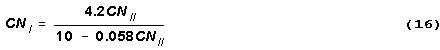
where CNII is the "moisture condition II" curve number for the
soil. CNII values are the normal tabulated curve numbers. Equations
11 to 14 estimate infiltration in inches for precipitation in inches.
Evapotranspiration Estimation: Four sources of daily evapotranspiration
(ET) are currently supported in CMLS98B. These are (1) actual ET values stored
in a data file, (2) estimated ET using daily pan evaporation data, (3) estimated
ET using the SCS Blaney-Criddle equations with historical or generated weather
data, and (4) estimated ET using the FAO Blaney-Criddle method and historical
or generated weather. Users can use other estimators outside of CMLS98B and
create "actual" ET files for use in this software. However, only the Blaney
- Criddle estimators can be used for Monte Carlo simulations. If you have
other estimators you would like to have incorporated, contact the authors.
(The methods used to estimate infiltration and flux of water passing the
current chemical depth make CMLS98B somewhat less sensitive than many crop
models to the distribution of daily evapotranspiration. In fact, CMLS98B is
sensitive only to the total ET between infiltration events. The distribution
of ET during that time period has no effect on the predicted flux of water
and chemical leaching.)
The basic concept with all of the ET estimators is to determine a reference
crop evapotranspiration value, ET0, and to relate ET0
to ET for the crop of interest by means of time dependent crop coefficients,
kCROP(t). That is
![]()
Values of kCROP(t) are obtained by linear interpolation between
tabulated kCROP(t') values (see details for Crop keyword of input
file) where t' is time measured from the date of planting.
For the pan evapotranspiration method, the reference crop evapotranspiration
is given by
![]()
where K is a pan constant (see ET Pan keyword of input file) and Pan(t) is
the pan evaporation amount on day t.
In CMLS98B the SCS Blaney-Criddle estimate of ET0 is calculated
by dividing the estimated monthly consumptive use by the number of days in
the month. Each day in the month then has the same ET0 value.
The consumptive use, U, for the month is obtained using the equation
![]()
where K is the consumptive use factor specified by the user, TF
is the mean monthly air temperature in degrees Fahrenheit, and p is the mean
monthly percentage of annual daytime hours (Jensen et al., 1990). A table
of values of p as a function of latitude from 0 to 64 degrees is built into
the software. The mean temperature is taken as the mean of the high and low
temperatures for each day in the month. The value of U calculated in equation
17 has units of inches.
The reference crop evapotranspiration for the FAO Blaney-Criddle method is
given by
![]()
where a and b are constants for a particular site (see ET Historical or ET Generated keywords of input file) and
![]()
Here p is the mean daily percent of annual daytime hours, and TC
is the mean air temperature in degrees Celsius (Jensen et al., 1990). The
mean temperature is taken as the mean of the high and low temperatures for
each day in the month. ET0 in equation 18 has units of mm.
Weather Generating: CMLS98B incorporates the stochastic model for
generating daily weather variables developed by Richardson and Wright (1984).
This software uses parameters derived from 10 or more years of daily weather
data at a site to generate daily rainfall, minimum and maximum temperatures,
and radiation characteristic of the site. WGEN enables one to examine the
behavior of chemicals at a site which has only limited historical data. It
is used to determine probability distributions for chemical fate
and transport at a particular site. Since future weather is not known at
the site, the model can be used to generate many independent sequences of
weather data typical of that site. By simulating the movement of the chemical
for each weather sequence, probability distributions can be determined for
soil - chemical - management systems of interest.
The publication of Richardson and Wright (1984) includes a program for extracting
the parameters needed to generate weather from historical weather data. The
format of these files is presented in the File Structure Section.
Irrigation: The irrigation module is capable of applying water in
two primary modes (in addition to using actual irrigation stored in a data
file). In the first case, irrigation is scheduled by the calendar. In this
mode, called periodic, a specified amount of water is applied at a specified
time interval during the irrigation season. In the second case, irrigation
is scheduled by the available water remaining in the root zone. During the
irrigation season, this demand mode of irrigation applies water whenever
the amount of available water in the root zone is decreased below some critical
depletion level. The amount of water to be applied is calculated by dividing
the amount of water needed to return the root zone to field capacity by the
application efficiency. If this calculated amount of water needed is less
than the minimum amount of water which can be applied by the system, the
minimum amount will be applied. For example, if 30 mm of water is needed
to return the soil to field capacity and the application efficiency is 75%
and the minimum amount which can be applied is 35 mm, the amount of water
applied would be 40 mm (30 mm/0.75 = 40 mm which is larger than 35 mm minimum).
If the application efficiency is 90%, 35 mm would be applied (30 mm/.90 =
33.3 mm which is less than the 35 mm minimum).
ASSUMPTION ABOUT IRRIGATION
1. All irrigation water infiltrates into the soil.